The Estimation of Mechanical Properties of Polymers from Molecular Structure ppt
Bạn đang xem bản rút gọn của tài liệu. Xem và tải ngay bản đầy đủ của tài liệu tại đây (1.16 MB, 21 trang )
The Estimation of Mechanical Properties
of
Polymers
from Molecular Structure
J.
T.
SElTZ
The
Dow
Chemical Co., Central Research,
1702
Building, Midland, Michigan
48674
SYNOPSIS
The use of semiempirical and empirical relationships have been developed to estimate the
mechanical properties of polymeric materials. Based on these relationships, properties can
be calculated from only five basic molecular properties. They are the molecular weight, van
der Waals volume, the length and number of rotational bonds in the repeat unit, as well
as the
Tg
of the polymer. Since these are fundamental molecular properties, they can be
obtained from either purely theoretical calculations or from group contributions. The use
of
these techniques by polymer chemists can provide a screening technique that will sig-
nificantly diminish their bench time
so
that they may pursue more creatively the design
of
new polymeric materials.
0
1993
John
Wiley
&
Sons,
Inc.
1.
INTRODUCTION
The purpose of this paper was to give polymer
chemists a technique for estimating the important
mechanical properties of a material from
its
molec-
ular structure. Hopefully, this will provide a screen-
ing tool that will significantly diminish their bench
time
so
that they may pursue more creatively the
design of new polymeric materials.
The important practical applications of polymers
are generally determined by a combination of heat
resistance, stiffness, strength, and cost-in short,
the engineering properties of a material. Other
properties may be of importance, but, if a polymer
does not have
a
balance of these properties, its
chances for commercial success are very limited. To
a large extent, these properties can be associated on
the molecular scale with the cohesive forces, the
molecular size, and the chain mobility. The approach
taken here is to relate molecular properties of the
repeat unit to the properties of the polymer. Repeat
unit properties can be obtained from group additivity
or
by simple calculations.
In the usual group contribution approach, little
consideration is given to the association between
molecular properties and macroproperties. The re-
Journal
of
Applied Polymer Science,
Vol.
49, 1331-1351 (1993)
0
1993
John Wiley
&
Sons,
Inc.
CCC 0021-8995/93/081331-21
sult is that for each property one wishes to calculate
a new table of fragments must be used. One of the
purposes of this study was to show that mechanical
properties can be estimated from a very few basic
molecular properties. Thus, we use semiempirical
means whenever available to make these associa-
tions. This has the effect of limiting the number of
tables of group contributions necessary to calculate
the basic properties, it simplifies the calculation
procedures, and it indicates to the theoreticians the
approximate form to which their theories may be
reduced.
Linking the mechanical properties to the molec-
ular properties of a material
is
the equation of state.
Thermodynamic relationships that involve the
pressure, volume, temperature, and internal energy
lead to the most fundamental equation of state. They
are expressed in the following form:
=
($)T
-
($),
(
$)T
=
(g)"
=
TaB
Here,
U
is
the internal energy,
S
is the entopy, and
P, V, and
T
have their usual meanings, and
a
=
1/
V[(dV)/(dT)]p and B
=
-V[(dP)/(dV)]p are
1331
1332
SEITZ
the thermal expansion and bulk modulus, respec-
tively.
For
mechanical properties below the glass tran-
sition temperature at constant temperature and very
small deformations, the entropy is assumed to be
constant. Above the glass transition temperature (in
the plateau region), the material behaves as a rubber
and the mechanical process can be assumed to be
mostly entropic. This leads to the following inter-
esting relationships:
Based on these simplifying assumptions, we will
proceed to develop estimates of the mechanical
properties of polymers.
II.
PRESSURE-VOLUME-TEMPERATURE
RELATIONSHIPS
Below
Tg,
P
=
TaB
-
-
(3)
(3,
A.
Volume-Temperature
(4)
It
has been found by a number of investigators that
there is a correspondence between the van der Waals
At
P
=
0,
TaB
=
Table
I
Thermal Expansion Data
VW
Polymer (cc/mol)
PE"
PIB
"
PMA"
PVA"
P4MP1
a
PVCb
PS
a
PMMA"
PP
"
PaMS
"
PET"
PDMPO"
PEMA"
PPMA"
PBMA"
PHMA"
POMA"
PVME"
PVEE"
PVBE"
PVHE"
PCLST"
PTBS"
PVT"
PBD
PEA^
PBA~
PCb
PEIS~
SAN
76/24'
20.46
40.90
45.88
45.88
61.36
29.23
62.85
56.10
30.68
73.07
94.18
69.32
37.40
66.33
76.56
86.79
107.25
127.71
34.38
44.61
54.84
75.30
72.73
104.67
74.00
56.11
76.57
53.78
136.21
94.18
28.0
56.1
86.1
86.1
84.2
62.5
104.1
100.0
42.1
118.1
192.2
120.0
54.1
114.1
128.2
142.2
170.3
198.4
58.0
72.0
86.0
114.0
138.5
160.0
118.0
100.1
128.2
88.7
254.3
192.2
140
202
282
304
302
355
373
378
258
453
339
480
188
338
308
292
268
253
260
231
218
199
389
405
388
251
224
384
423
324
P
(gm/cc)
0.97
0.93
1.21
1.18
0.84
1.36
1.03
1.15
0.88
1.02
1.30
1.03
1.12
1.11
1.07
1.06
1.03
1.00
1.02
1.00
0.98
0.99
0.97
0.95
1.02
1.09
1.11
1.07
1.20
1.33
2.01
1.44
2.70
2.12
3.83
1.75
2.50
2.13
3.43
2.40
1.62
2.04
2.00
3.09
3.63
4.12
4.40
4.15
2.16
3.03
3.9
3.75
1.45
2.58
1.59
2.80
2.60
2.27
2.65
2.00
5.31
5.86
5.60
5.83
7.61
4.85
5.50
4.90
8.50
5.40
4.42
5.13
7.05
5.40
5.75
6.05
6.80
6.00
6.45
7.26
7.26
6.60
4.97
5.90
3.78
6.10
6.00
4.87
5.35
4.55
a
Ref.
5.
All the densities reported from this reference are cited at the glass transition temperature.
Ref.
6.
Internal data of The
Dow
Chemical
Co.
ESTIMATION
OF
MECHANICAL PROPERTIES
OF
POLYMERS
1333
volume and the molar volume of polymers.'-3 Van
der Waals volume is defined
as
the space occupied
by a molecule that is impenetrable to other mole-
cules.' Van der Waals radii can be obtained from
gas-phase data4 and bond lengths can be obtained
from X-ray diffraction studies. Using these data, the
volume may be calculated for a particular molecule.
Bondi' and Slonimskii et a1.2 calculated group con-
tributions to the van der Waals volume for large
molecules and demonstrated the additivity.
Since polymers consist of long chains, which
dominate their configuration as they solidify into a
glass, one might expect that they would pack quite
similarly regardless of their quite different chemical
natures. To determine
if
this hypothesis is correct,
it is necessary to obtain the molar volume at some
point where the polymers may be expected to be in
the same equivalent state and to compare them with
a measurable molecular volume such as the van der
Waals volume. Two temperatures are of interest:
absolute zero and the glass transition temperature.
At absolute zero, all thermal motion stops and the
material is in a static state. The glass transition is
considered to be the point where the material begins
to take on long-range motion and the properties are
no longer controlled by short-range interactions.
In Table I, we have compiled the densities and
the thermal coefficient, in terms of the slope of the
volume-temperature curve, from several sources in
the literature. We have then calculated the volume
at the glass transition temperature and at
0
K
using
a straight-line extrapolation of the data. The results
are tabulated in Table
11.
The data from Table I1 is
then plotted as van der Waals volume vs. the molar
volumes and
fit
with a straight line that was forced
through zero. The results of these plots are shown
in Figure l(a)-(c).
It is apparent from the data that there is a rea-
sonably good
fit
between the molar volumes at the
selected equivalent states. To determine the validity
of the approximation, thermal expansion data rang-
ing from room temperature down to
14
K
were ob-
tained from the work of Roe and Simha.7 A fifth-
degree polynomial was
fit
to the data (see Fig.
2)
and the volume-temperature curves were then ex-
tracted from the data by using eqs.
(
7)
and
(8)
:
CY
=
aT5
+
bT4
+
cT3
+
dT2
+
eT
+f
(7)
Vog
=
V298exp
-
(8)
V
=
Vogexp
J
CY
dT
(9)
0
Table
I1
Molar Volumes
VW
VK
VOK
vor
Polymer (cc/mol) (cc/mol) (cc/mol) (cc/mol)
PE
PIB
PMA
PVA
P4MP1
PVC
PS
PMMA
PP
PaMS
PET
PDMPO
PBD
PEMA
PPMA
PBMA
PHMA
POMA
PVME
PVEE
PVBE
PVHE
PCLST
PTBS
PVT
PEA
PBA
SAN
76/24
PC
PEIS
20.5
40.9
45.9
45.9
61.4
29.2
62.9
56.1
30.7
73.1
94.2
69.3
37.4
66.3
76.6
86.8
107.3
127.7
34.4
44.6
54.8
75.3
72.7
104.7
74.0
56.1
76.5
53.8
136.2
94.2
28.9
60.1
69.4
72.7
100.5
45.4
100.9
86.7
47.5
115.2
147.6
116.4
44.1
102.6
119.2
134.5
165.2
184.4
54.0
72.2
87.4
115.6
143.3
171.7
117.3
88.3
109.0
84.6
220.3
145.0
28.2
58.4
62.9
67.2
90.7
38.7
91.2
78.6
44.1
102.3
137.1
104.6
42.0
90.7
104.9
117.5
145.2
165.0
50.7
67.2
80.1
107.1
135.5
155.0
110.0
81.4
102.1
76.9
197.8
132.5
26.9
53.6
55.9
57.5
81.4
35.1
79.6
68.2
38.3
86.4
119.0
86.9
36.9
81.9
96.7
109.6
134.5
168.7
44.3
60.1
73.8
100.7
116.6
133.4
100.0
73.0
91.7
68.0
162.8
116.6
where
a,
b,
c,
d,
e,
and fare coefficients from the
fifth-degree polynomial
fit,
and
T
=
temperature,
K.
The thermal expansion curves show very clearly
the various transitions due to thermally activated
molecular motions. However, when these data are
integrated to give the volume-temperature curves,
these transitions are smeared out into what appears
to be a nearly continuous function as can be seen
in Figure 3(a)-(c).
The results can be
fit
with a
T1.5
relationship as
predicted by free-volume theory? However, from 150
K
to the glass transition temperature, the data can
be very nicely approximated by a straight line. These
relationships are shown by the solid and dashed lines
in Figure
3
(a)
-
(c) and are described by eqs.
(
10)
and
(
11).
Table
I11
summarizes the data for the six
different materials:
rp
1.5
0
40
80
120
van
der
Waals
Volume, cc/mol
SloDe
=
1.42
'
Std: dev.
=
7.84
Correlation index
=
0.995
0
0
40
80
120
van
der
Waals Volume, cc/mol
0
40
80
120
van
der
Waals
Volume, cdmol
Figure
1
(a)
Van der Waals volume vs. molar volume at the glass transition temperature;
(b)
van der Waals volume vs. molar volume for the glass
at
0
K;
(c)
van der Waals volume
vs. molar volume
of
the rubber at
0
K.
T
T8
where
T,
=
glass transition temperature,
K,
and
6
=
V,
-
Vog
=
0.15.
Based on the results from these data, we feel jus-
tified in defining the slope of the volume-tempera-
ture curve as a constant over a wide range of tem-
peratures. This approximation allows the data to be
described by the Simha-Boyerg-type diagram as
shown in Figure
4.
Further, the volume can be de-
scribed as being distributed in three parts:
(1)
the
van der Waals volume
or
the volume considered to
be impenetrable by other molecules;
(
2)
the packing
v=
6-+
vog
(
l1
)
ESTIMATION
OF
MECHANICAL PROPERTIES
OF
POLYMERS
1335
3e-04
?c
2e-04
\
4
h
2i
aJ
le-04
Oe+00
PS
i
AMS
0
PC
x
PPO
0
POMS
I
100
200
300
400 500
Temperature,
K
Figure
2
Thermal expansion data of
Roe
and Simha7
fit
with a fifth-degree polynomial.
volume that reflects the shape and long-chain nature
of the molecule; and
(3)
the expansion volume that
is due to thermal motion of the molecules.
Using the values generated from the straight-line
fit
of the data in Figure
1
(a)
-
(c)
,
the slope and the
intercept of the volume-temperature curve can be
established for amorphous polymers in both the
glassy and rubbery state:
The thermal expansion coefficient can thus be ob-
tained by differentiating eqs 12(a) and (12b) and
by using its standard definition:
1
(13b)
1
dV
ffr
=
v
dT
=
(T
+
4.23Tg)
The density can be estimated from the molecular
weight of the repeat unit divided by the molar vol-
ume:
M
P=v
B.
Pressure-Volume
The pressure-volume-temperature response in
polymers can be determined by several molecular
factors. They include intermolecular potential, bond
rotational energies bond, and bond-angle distortion
energies. The bond-angle distortion energies are
important in anisotropic systems where aligned
chains are subjected to a stress
or
pressure. In iso-
tropic glasses where the bonds are randomly ori-
ented, the properties are controlled by rotational and
intermolecular potentials. In the following sections,
we will separate these into entropy and internal en-
ergy terms and then try to relate this to the molec-
ular structure using properties that can be related
to the molecular structure either by direct calcula-
tion
or
through quantitative structure property re-
lationships (QSPR)
.
In a perfect crystalline lattice, specific short-range
and long-range interactions can be accounted for,
but amorphous polymers by their very nature do not
fit
these computational schemes. Several attempts
have been made at using quasi-lattice models to de-
scribe the equation of state.1°-16 Most of these are
quite limited and need additional information about
reduced variables
or
lattice types. Computer models
using molecular mechanics techniques have been
devised based either on an amorphous cell, which is
generated from a parent chain whose conformation
is generated using rotational isomeric-state calcu-
lations,
l7
or
on computer models that also start from
RIS configurations and generate radial distribution
functions." Both approaches use an l/r6 potential
function to calculate the state properties.
1336
SEITZ
Temperature,
K
0.199T
+
93.6
0.929~10.~
T15+
94.86
I
;
220
\
0
V
215
n
B
3
210
2
205
0
200
I
0
100
200
300
400
500
Temperature,
K
.0402T
+
200.79
0 1605~10-~
T15+
204.2
264
I
\
;
V
262
B
=I
I
260
L
cp
0
I
E
258
0
50
100
150
200
250
300
Temperature,
K
.0144T
+
258.0
0.690~10”
TI5+
258.8
Figure
3
(a) Calculated volume-temperature data for polystyrene; (b) calculated volume-
temperature data for polycarbonate;
(
c
)
calculated volume-temperature data for
poly
[
N,N’(p,p’-oxydiphenylene)pyromellitimide]
(PI).
ESTIMATION
OF
MECHANICAL PROPERTIES
OF
POLYMERS
1337
L
m
2
Table
I11
Molar Volume Calculated from the Data from
Roe
and Simha'
Volume
I111IIIIl
~
PS
93.6
94.85
373 62.85 1.49
1.51
PC
200.8
204.2
423 136.2 1.47 1.50
PPO
106.2
107.4
475 69.32
1.53
1.55
POMS
109.8
110.9
409 74.00 1.48 1.50
PaMS
93.6
112.9
443 73.07 1.53
1.55
PI
258
258.8
630 185.2 1.39 1.40
CHDMT
215.5
218.7
365 149.2 1.44 1.46
Here, we will divide the polymer molecule into
suitable submolecules (repeat units) that will then
be assumed to be surrounded by a mean field at a
distance
r.
We will also assume that the volume of
the repeat unit can be described in terms
of
its van
der Waals volume. The field potential will be de-
scribed by a Lennard-Jones" potential function:
Thus, the molar volume is related to the intermo-
lecular distance
r
as follows:
Nr
C
v=-
where
N
is Avogadro's number and
C
is a constant
that corrects
for
the geometry of the submolecule.
On substituting the ratio of the volumes, one arrives
at the following relationship between volume and
intermolecular distance:
3
-
V
=
(p)
VO
The total potential energy of a system containing
N
repeat units is
U
=
Ne and at the minimum
Uo
=
Neo
(18)
Equations (15) and
(18)
combine to define the con-
tribution to the internal energy
U
from the inter-
molecular potential:
u=
uo[2(;)'-(;)l] (19)
Taking the partial of
U
with respect to V and sub-
stituting into the thermodynamic equation state for
P
below the glass transition temperature yields
p
=
(
g)T
-
y
[
(;
)'
-
(+)'I
(
20)
At zero pressure and constant temperature,
where Vis the molar volume, cc/mol;
V,,
the molar
volume at the temperature of interest, cc/mol; Vo,
the molar volume at the minimum in the potential
well; and
Uo,
is the depth of the well
The bulk modulus is defined by -V
[
(dP)/
(dV)]T. Taking the derivative of eq. (22) and mul-
tiplying by V gives
1.6OVm
5
1.45Vh
E
0
I
1
Packing
Volume
a
8
Van
der
Waal's
-
Tg
Temperature,
K
Figure
4
Volume-temperature diagram.
0
1338
SEITZ
B=?[(Y)
5vo
-(?)'I
(23)
Haward2' used a form of this equation to predict
the relationship between the volume and the bulk
modulus of poly
(
methyl methacrylate).
Pressure-volume data were obtained from
Kaelble'l was
fit
to eq.
(
23)
using regression analysis
to solve for the value
of
Uo.
The factor
Vo
was as-
sumed to be the molar volume of the glass at
0
K
(
1.42
V,,,) .
The solid line shows the
fit
to the data in
Figure 5(a)-(c).
2e+09
E
Y
sf
.
v1
0
le+09
2-
2
2
v)
a
Oe+
0
0
94
96 98
100
Molar
Volume,
cc/mol
2e+09
E
r
z
.$
le+09
$
E:
80 82 84 86 88
Molar
Volume,
cc/mol
2e+09
E
Y
a
\
yl
a,
C
x
le+09
a
2
6
Oe+00
yl
yl
41 42 43 44
45
46
Molar
Volume, cc/mol
Figure
5
(a) Pressure-volume dataz1
for
polystyrene;
(b)
pressure-volume dataz1
for
poly
(
methyl methacry-
late
)
;
(c
)
pressure-volume
data21
for
poly (vinyl chloride).
Table IV
Volume Data
Uo
as
Calculated from the Pressure-
PS
7.3034 7.1234
3.4334 2.15
PMMA
5.0934
4.7934
2.9334 1.74
PVC
3.3134
3.0934
1.7234 1.92
Table
IV
shows the values of
Uo
that were ob-
tained from the
fit
of the data along with the molar
cohesive energy as calculated from the data of Fe-
dors22 and van der Waals volume from Bondi' and
Slonimski et a1.2 as compiled in Ref.
23.
The ratio
of
Uo
to the cohesive energy
for
these three polymers
averages
1.94,
or
approximately
2.
We will show later
from the analysis of the mechanical properties that
this ratio,
Uo/
Ucoh,
is indeed very close to
2.
111.
MECHANICAL
PROPERTIES
A.
The Modulus and the Stress-Strain Curve
1.
Volume-Strain Relationships
The important moduli for engineering applications
are the shear modulus
G
and the tensile modulus
E.
They are related to the bulk modulus
B
in the fol-
lowing manner:
E
=
3B(1
-
2v)
=
2G(1
+
U)
(24)
E
and
G
may be evaluated from the bulk modulus
using eq.
(23)
if the value
u
(Poisson's ratio) is
known. Poisson's ratio is defined as the ratio of the
lateral contraction in the
y
and
z
directions as a
tensile stress is applied in the
x
direction and it ac-
counts for the change in volume during the defor-
mation process. Stress and strain can be introduced
into the calculations as volume changes
by
using the
following relationships:
-
de,
+
dey
+
dez
(25)
dV
V
ESTIMATION
OF
MECHANICAL PROPERTIES
OF
POLYMERS
1339
where the subscripts
x,
y
,
and
z
denote the stresses
and strains in three principal directions.
In the case of a material being stretched uniaxially
in the
x
direction, eq.
(25)
can be solved for the
strain in terms of Poisson's ratio and the volume by
using eq.
(27)
:
e=Jde=J
v,
(1
-
2v)V dV
(28)
1
V
Using the results of eqs.
(26)
and
(28)
with the
assumption that the stress is zero in all directions,
except in the
x
direction, eq. (22) can now be solved
in terms of stress and strain where
V,
is the volume-
dependent strain:
Similarly, substituting eqs.
(
24)
and
(28)
into eq.
(
23
)
,
the tensile modulus is obtained
E
=
24(1
-
2v)Ucoh
[
5-
;
-
3-
:]
(30)
The value of
V,
can be estimated from van der
Waals volume and the glass transition temperature
using eqs.
(
lo),
(ll),
or
(12),
and
Uo
may be esti-
mated using the approximation that it is two times
the cohesive energy. However, without a relationship
between Poisson's ratio and the molecular structure,
we are unable to calculate the tensile
or
shear
moduli.
2.
Poisson's
Ratio.
Our model as presently constituted does not contain
any information about the directional properties of
the system. However, just as the bulk modulus varies
as
1
/V
in eq.
(23),
one might expect that a simplified
unidirectional (tensile) moduli would vary as the
area being stressed. Using this analogy, Poisson's
ratio can be equated to
E/B
from eq.
(25).
The
result of this relationship can be stated as follows:
v
=
0.5
-
kfi
(31)
(32)
where
1,
is the length of the repeat unit in its fully
extended conformation and
NA
is
Avogadro's num-
ber. The fully extended conformation corresponds
to the all-trans-conformation and can be calculated
by assuming ideal tetrahedral bonding around the
carbon atoms in the polymer backbone and using
simple trigonomeric relationships. Table
V
gives the
calculated
A
for a number of polymers for which we
have data.
The data from Table
V
is plotted in Figure
6
and
is represented by the circular symbols. The line in
Figure
6
was obtained by fitting the data to a square-
root argument using regression analysis. The sta-
tistical
fit
represented by eq.
(33)
has a standard
deviation of 0.019 and a correlation index of 0.998:
(33)
To estimate the stress-strain relationship as a func-
tion of temperature, we must have both Poisson's
ratio and the volume as a function of temperature.
The temperature-volume relationships can be cal-
culated from eq.
(
12a).
A=-
vw
NA
1,
v
=
-2.37
X
106fi
+
0.513
Table
V
Cross-sectional Area
Poisson's Ratio and Molecular
M
o
1
e c
u
1
a r
Cross-sectional
Poisson's Area
Polymer Ratio (cm2
x
10-l~)
Polycarbonate
PS
ST/MMA
35/65
Poly(p-methyl styrene)
SAN
76/24
PSF
PDMPO
PET
POMS
Arylate
1
:
1
:
2
Phenoxy resin
PMMA
PTBS
PVC
Poly(amide-imide)
0.401"
0.354"
0.361"
0.341"
0.366"
0.441'
0.410b
0.430b
0.345"
0.433"
0.402"
0.371"
0.330"
0.385"
0.380"
19.8
41.1
38.0
48.4
33.8
20.1
27.6
14.0
46.4
19.2
19.2
37.2
68.5
18.5
18.6
The value
A
can be thought of as the molecular
cross-sectional area and is defined here as the area
of the end of a cylinder whose volume is equal to
the van der Waals volume of the repeat unit and
has a length of the repeat unit in its all transcon-
figuration:
a
Internal data of The Dow Chemical Co. Poisson's ratio was
measured using an MTS biaxial extensometer no. 632.85B-05 in
conjunction with an MTS
880
hydraulic testing machine. The
tests were performed under the conditions
of
ASTM D638, using
type
1
tensile specimens. The crosshead speed was
0.2
in./min.
All samples were compression-molded and then annealed at
(T,
30
K)
for
24
h.
Data obtained from Ref.
24.
1340
SEITZ
0.50
0.45
0
m
In
c
0
cn
In
0
IL
,-
c
0.40
,-
0.35
0.30
I I I I I
1 1 1
1
0 10 20 30 40 50 60 70 80 90 100
Molecular Cross-sectional Rrea,
cmZ
x
1016
Figure
6
Poisson's ratio as
a
function
of
molecular area.
Poisson's ratio increases very slowly as a function
of
temperature to within
20"
of
the glass transition
temperature with only very minor deviations due to
low-temperature transitions. Just above the glass
transition temperature, Poisson's ratio is assumed
to approach
0.5
so
that the volume is conserved in
the rubbery state. Based on the data and the previous
assumption, a fitting function was developed to es-
Table
VI
Poisson's
Ratio
as
a
Function
of
Temperature
PC
PS
PMMA PVT ST/MMA PVC POMS
T
V
T
V
T
V
T
V
T
V
T
V
T
V
173 0.386 173 0.352 173 0.339 297 0.341 296 0.361 173 0.364 173 0.348
193 0.390 193 0.352 193 0.340 313 0.342 313 0.364 193 0.371 193 0.344
213 0.395 213 0.348 213 0.342 333 0.350 333 0.368 213 0.373 213 0.344
233 0.398 233 0.353 233 0.346 353 0.359 353 0.376 233 0.379 233 0.346
253 0.401 253 0.353 253 0.351 173 0.327 173 0.339 253 0.382 253 0.342
273 0.402 273 0.354 273 0.358 193 0.328 193 0.340 273 0.383 273 0.340
293 0.401 296 0.354 296 0.361 213 0.328 213 0.342 293 0.385 293 0.345
313 0.399 313 0.355 313 0.364 233 0.332 233 0.346 313 0.388 313 0.343
333 0.400 333 0.356 333 0.368 253 0.334 273 0.358 333 0.405 333 0.348
353 0.399 353 0.359 353 0.376 273 0.337 253 0.351 354 0.500 353 0.352
373 0.398 373 0.500 387 0.500 373
0.500
382 0.500 373 0.370 373 0.370
393 0.398
413 0.401
423 0.500
Poisson's ratio was measured using an MTS biaxial extensometer no. 632.85B-05 in conjunction with an MTS 880 hydraulic testing
machine. The tests were performed under the conditions of ASTM D638 using type
1
tensile specimens. The crosshead speed was
0.2
in./min. All samples were compression-molded and then annealed at
(T,
30
K)
for
24
h.
ESTIMATION
OF
MECHANICAL PROPERTIES
OF
POLYMERS
1341
timate the relation between temperature and Pois-
son’s ratio. Table
VI
gives Poisson’s ratio as a func-
tion of the temperature for seven polymers. The
fit-
ting function for these data is as follows:
T
UT
=
UO
+
50
-
{
1.63
X
Tg
where
VT
is Poisson’s ratio at temperature
T,
and
vo
can be calculated from substituting in the value at
room temperature for
uT,
which can be determined
from eq.
(33).
The results of using this fitting equa-
tion are shown in Figures
7
(a)
-
(c
)
.
3.
Tensile
Modulus
Employing Poisson’s ratio and the experimental
tensile modlui,
Uo
was calculated from eq.
(30).
The
average of the ratio
of
Uo/Ucoh
was
2.06
for all
18
polymers in Table
VII.
The final column of the table
shows the calculated values of the tensile modulus
using
Uo
=
2.06
Ucoh.
When compared with the ex-
perimental data (see Fig.
8)’
the results give a cor-
relation index of 0.988 and a standard deviation
of
the regression of
0.334.
The final form
for
the room-temperature modulus
in units of Pascals is
E
=
24.2
X
106Uc,h
Tg
[
5(
9.47T
+
Tg
)”
-
3(
9.47?+
Tg
r]
(35)
The temperature modulus curve can be calculated
by substituting the volume and Poisson’s ratio tem-
perature relationships from eqs.
(11)
and
(33)
into
eq.
(30).
The results
of
this calculation are shown
for polystyrene in Figure 9.
B.
Deformation Mechanisms
There are two dominant modes of deformation in
polymers: shear yielding and crazing. Although nei-
ther process is entirely understood at the molecular
level, it is the intent here to attempt to correlate
these mechanisms with the molecular structure us-
ing existing theories and empirical relationships.
0.50
0.48
0.46
0.44
0.42
0.40
I
1
0.30
0.32
150
1
200
250
300
350
400
2
Temperature,
K
n
cn
0.46
I
0.44’
0.40
0.38‘
Data
-
Calculated
0.32‘
0.30.
.I
#
150
200
250
300 350
400
1
Temperature,
K
0.46
0.304
.
,
.
,
.
,
.
,
.
,
.
150
200 250 300 350
400
1
Temperature,
K
Figure
7
(a) Poisson’s ratio as a function of tempera-
ture for poly (methyl methacrylate)
;
(b) Poisson’s ratio
as
a
function of temperature for polystyrene; (c) Poisson’s
ratio as a function of temperature for polycarbonate.
1342
SEITZ
Table
VII
Tensile Modulus Data
Expt Calcd
Modulus
VW
MW
1,
T,
Ecoh
X
Poisson's Modulus
Polymer (GPa) (g/mol) WmoU (cm)
(K)
(i/mol) Ratio (GPa)
O-CIST 4.0b 72.7 138.5
2.21 392 5.19
0.32 4.16
ST/MMA 65/35 3.5b
58.0
101.4
2.21
373 3.61 0.36
2.91
ST/aMS 52/48 3.Sb 65.7
111
2.21
408 4.16
0.33 3.48
PAMS 3.1b 68.5
118
2.11
443 4.31 0.32
3.1
PC
2.3 136.2
254
10.75 423 9.24
0.40 2.27
PS
3.3b
62.9
104
2.21
373 4.03 0.35 3.20
PMMA
3.2b 56.1 100
2.11 378 3.38
0.37 2.62
SAN 76/24
3.8b
51.3
84.6
2.21
378 3.79 0.37
3.19
PPO
2.3" 69.3 120
4.6
484 4.47 0.41
1.95
PET
3.0" 90.9
192
10.77
346 12.06 0.43
3.11
PSF
2.5'
234.3
443
18.3 463 19.20
0.44 1.66
PVC
2.6" 28.6 62
2.55 358 1.99
0.39 2.52
PTBS 3.0b
104.7
160
2.21
405 4.75 0.33
2.61
PHEN 2.3b 162.6
277
10.70
363 12.50 0.40
2.59
PES 2.6d 111.9 224.1
10.40
503 9.32 0.42
2.24
PEC
1
:
1
2.3b 194.7 596
2.51 448 23.50
0.44 2.44
ARYL
1
:
1
:
2 2.ld 338.7
644 31.20 463 28.50
0.44 1.71
PVT 3.1 74.0
118
2.21
388
4.50
0.34 3.26
a
All
data for cohesive energy was obtained from Fedors (see Ref.
22)
with the exception of the value of
SO2
where
a
value of
26,000
Internal data of The Dow Chemical
Co.
The data were obtained under conditions of ASTM
D-638
using type
1
tensile bars and a
was used.
200
:
1
extensometer.
'
Ref.
25.
Ref.
26.
50
45
41)
35
31)
25
2D
15
1D
05
OD
I
I
I
I
I
1
OD
05
1D
15
21)
25 30 35 4D 45 51)
Calculated
Tensile
Modulus,
GPa
Figure
8
Comparison
of
experimental modulus with calculated tensile moduli.
ESTIMATION
OF
MECHANICAL PROPERTIES
OF
POLYMERS
1343
Data
calculated
Temperature,
K
Figure
9
Tensile modulus
of
polystyrene as a function
of
temperature.
1.
Shear Yielding
There have been many attempts to describe the yield
strength from the molecular point
of
None
of these relates well to basic molecular parameters.
However,
a
good correlation between modulus and
yield strength has been noted by several research-
er~.~~-~~ Brown35 suggests the following as an ap-
proximate equation for the yield point:
where the value
of
K
is
a constant
for
amorphous
linear polymers,
G(
P,
T)
is the shear modulus that
depends on
P
and
T,
and
V,
and
Eo
are material
parameters involving an activation volume and a
reference strain rate. Table VIII gives the tensile
modulus and the tensile yield strength of a number
of materials rather than the shear modulus.
On the assumption that the time-dependent term
is much smaller than the first term of eq. (36), the
data from Table VIII were
fit
by
a straight line using
regression analysis. The results of the
fit
are shown
in Figure
10.
The
fit
of the line to the data gives a
standard deviation of 0.968 MPa and a correlation
index of 0.976. It
is
interesting to note that the
semicrystalline polymers as well as the amorphous
polymers can be represented in this way, thus mak-
Table
VIII
Tensile Modulus and Yield Strength
Tensile Yield
Modulus Strength
Polymer (GPa) (MPa) Ratio
HDPE"
LDPE"
PP
a
PSb
PVC
a
PTFE"
PMMA~
PCb
NY6/10d
PET"
CA"
CLST~
SAN~
PPO
PHEN"
PSF"
PES'
NY
6"
NY
6/Sa
1.0
0.2
1.4
3.3
2.6
0.4
3.2
2.3
1.2
3.0
2.0
4.0
3.8
2.3
2.3
2.5
2.6
1.9
2.0
30
8
32
76
48
13
90
62
45
72
42
90
83
72
66
69
84
50
57
0.030
0.040
0.023
0.023
0.019
0.033
0.028
0.027
0.038
0.024
0.021
0.025
0.022
0.031
0.029
0.028
0.032
0.263
0.029
a
Ref.
24.
bInternal data of The Dow Chemical Co. obtained from a
biaxial test conducted in simultaneous tension and compression.
The yield point was obtained by extrapolation using a Von Mises
criteria.
Ref.
36.
Ref.
34.
1344
SEITZ
0.09
0.08
0.07
0.06
0.05
0.04
0.03
0.02
0.01
ing the relationship universal for all p0lymers.3~
Equation
(29)
can now be rewritten in terms of ten-
sile stress as follows:
-
-
-
-
-
-
-
-
-
(37)
The other material constants change to account for
the tensile component of stress rather than for the
shear component. The temperature dependency of
the yield stress can be determined from the tem-
perature dependency of the modulus.
2.
Crazing
Because the stress to initiate a craze depends on
local stress concentrators,
it
is very difficult to an-
alyze from a molecular viewpoint. In fact, as of yet,
there appears to be no quantitative method of re-
lating crazing to molecular structure.
However, the relationship between materials that
carze and materials that shear yield has been cor-
related with entanglement spacing by Donald and
Kramer.37p3s Using their results, a criterion can be
established, based on the contour length of the en-
tanglement to predict
if
a material will craze
or
shear
yield.
If
the contour length turns out to be greater
than approximately
200
A,
the material will mostly
likely craze.
If
the contour length is less than
200
A,
then shear yielding
is
expected. The contour
length can be calculated from entanglement spacing
that can be obtained from dynamic mechanical data
(see section on entanglements). Wu3’ correlated the
crazing stress
(I,
with the entanglement density as
follows:
3.
Brittle Fracture
At sufficiently low temperatures, all glassy polymers
behave in a brittle manner, but as the temperature
approaches the glass transition temperature, they
generally become ductile. The tensile stress to frac-
ture at which the material exhibits no ductile failure
mechanisms, i.e., crazing
or
shear yielding, is termed
the brittle stress. Usually, this stress is never real-
ized, except in highly cross-linked systems
or
at ex-
tremely low temperatures, because some ductile
0.10
1
I
I
I
I
I
I
I
I
I
0
0.0
0.5
1.0
1.5
2.0
2.5
3.0
3.5
4.0 4.5
5.0
Tensile
Modulus,
GPa
Figure
10
Tensile modulus
vs.
tensile yield strength.
ESTIMATION
OF
MECHANICAL PROPERTIES
OF
POLYMERS
1345
process interferes before this limiting value is
reached. However, it can be used as a base line to
establish the maximum stress that a material can
withstand. Therefore,
if
a shear yield stress is cal-
culated that
is
higher than this value, brittle fracture
can be expected to occur.
Vincent4' attempted to quantify this number for
a series of different polymeric materials and related
the brittle stress to the number of backbone bonds
per unit area. Data from Vincent as well as data
from this laboratory along with pertinent molecular
information are shown in Table IX. The number of
bonds/cm2 are calculated from the following
expression:
NL
V
nB
=
-
(39)
where
nB
is the number of bonds;
N,
Avogadro's
number;
l,,
the length of the repeat unit; and
V,
the
molar volume. The theoretical brittle stress is then
the number of bonds times the strength of an in-
dividual bond. The real strength of the material is
much less because defects exist within the material
that result in very highly stressed local areas. If we
Table
IX
Brittle Strength
of
Polymers
plot
nB
against the measured brittle strength, the
result is a straight line. The slope
of
the line rep-
resents the strength per bond.
The results of a linear regression analysis of the
data in Table IX is shown in Figure
11.
The straight-
line
fit
to the data has a standard deviation of
regression of 16 MPa and a correlation index of
0.982.
The force to break a
C-C
bond is estimated to
be 3-6
X
10-9N.41942
The slope of the brittle strength
line is
0.038
X
10-9N.
Thus, only about
1%
of the
bonds are involved in the fracture process in amor-
phous materials
or,
in other terms, the stress con-
centration factor appears to be about
100
for a large
number of materials. The brittle strength for amor-
phous polymers can be calculated from the following
equation:
This approach can be used to estimate the theoret-
ical strength of a fully oriented polymer as well as
a thermoset. As an example using this correlation,
we estimate the strength of a fully extended linear
Brittle
TB
TB
1,
VW
No. Bonds Strength
Polymer
(K)
(K)
(4
(cc/mol)
x
10-14 (MPa)
PE"
P4MP"
PVC"
PSb
PMMA"
PP"
PET"
PC"
P-CLST~
PTBS~
SAN~
PVTb
PMO"
PPE"
PTFE"
PES"
NY"
PB-1"
147
305
358
373
387
264
345
423
389
405
353
216
380
255
200
113
503
324
77
243
193
298
333
153
173
133
298
298
298
173
298
213
173
77
93
173
2.53
1.98
2.55
2.21
2.11
2.17
10.77
10.75
2.21
2.21
2.21
1.92
2.00
2.16
2.17
2.6
10.4
17.3
20.4
61.3
28.6
62.8
56.1
36.6
90.8
136.2
72.7
104.6
74.0
16.0
53.7
51.1
40.9
30.7
107.2
141.2
4.94
1.26
3.56
1.34
1.46
2.83
4.78
3.24
1.16
0.81
1.14
4.6
1.42
1.79
2.02
3.22
3.70
4.67
160
53
142
41
68
98
155
145
41
31
46
216
62
58
81
117
148
179
a
Ref.
40.
Internal data
of
The Dow Chemical
Co.
All brittle strength data was obtained at room temperature using a crosshead speed
of
0.2
in./min with a type
B
tensile specimen under conditions of ASTM D638.
SEITZ
I
I
0
e
I 2
3
4
5
6
Number
of
bonds/cm2
H
I
8-14
Figure
11
bonds.
Brittle strength
vs.
number
of
backbone
polyethylene polymer to be
13.2
GPa. In practice,
about
5
GPa has been achieved and the value of
13
GPa has been extrapolated from experimental data.
This agreement points out the utility of this ap-
proach in estimating the strength of ordered poly-
mers.
The effects of molecular weight on the strength
of glassy polymers
is
to increase from near zero at
very low molecular weights to a constant value at
high molecular weights. Fl~ry~~ showed that a plot
of tensile strength vs. the reciprocal molecular
weight gave a straight-line relationship for cellulose
acetate. Gent and Thomas44 derived the maximum
value for the number-average molecular weight at
zero flexural strength
(Mf)
.
Kinloch and Young45
listed a few values for
Mf
and six have been plotted
against the entanglement molecular weight
(Me).
As can be seen from Figure
12,
the result is a
fairly good straight-line relationship between Mf and
Me
with a slope of
0.296.
Assuming that the tensile
strength and the flexural strength go to zero at the
same molecular weight, a function of molecular
weight can be written as follows:
C.
Entanglements and Mechanical Properties
We have already noted the dependence of crazing
on the entanglement length. Many other properties
also depend on the entanglement spacing such as
the modulus in the plateau region above the glass
transition, the viscosity, the fracture strength, and
the glass transition.
Calculating shear and tensile properties above the
glass transition is more difficult because polymers
are viscoelastic and therefore very time-dependent.
Our models are static models and therefore no in-
formation about time dependency can be obtained
from them. However, we can estimate the shear
modulus in the plateau zone from the analogy with
rubber elasticity, where
Ge
is
the equilibrium mod-
ulus;
r,
the density;
R,
the gas constant, and
T,
the
absolute temperature:
PRT
Ge
=
-
Me
This, of course, can only be obtained if the plateau
zone were constant. In real polymers, there is almost
always a slope,
so
that
it
is difficult to determine at
what point to take the data. Since we are dealing
with a viscoelastic material, the true equilibrium
modulus cannot be obtained. The general approach
is to use the viscoelastic equivalent called the pseu-
doequilibrium modulus,
Gb,
which can be obtained
from dynamic data by integrating the loss modulus,
G",
from dynamic mechanical data. The author has
bound that the value of the storage modulus
G'
ob-
2oooo
r
/
where
uf
is
the stress to fail;
ab,
the stress calculated
from eq.
(40);
and
M,
the number-average molecular
Mf,
gdmole
Figure
12
Molecular weight at zero flexural strength
weight.
(M,)
vs.
entanglement molecular weight.
ESTIMATION
OF
MECHANICAL PROPERTIES
OF
POLYMERS
1347
Table
X
Entanglement Data
Polymer
v,
(cc/mol)
PE
a
HPIP"
PBD
51/37/12'
NY66b
POE"
PSF"
PVF2
PEC
1
:
1"
PEC
1
:
2"
NYb
PC'
POM
PET^
APA~
PHEN~
PETG~
PBDcis"
PBDvinyl"
PPO"
SAN
50/50"
SAN
63/37'
S/MMA
35/65'
PTFE~
PDMS~
PEMA~
PVAC
"
SAN
76/24'
PIB"
SAN
71/29'
PMMA'
SAN
78/22'
PAMS"
SMA
67/23'
SAA
92/8'
SMA
91/9'
SAA
87/13'
SMA
79/21'
PS'
P2EBMA"
P-PVT'
P-BRS'
PMA~
PHMA"
TBS'
28.0
192.0
69.0
54.0
226.0
246.0
44.0
442.0
64.0
596.0
938.0
113.0
254.0
30.0
288.0
684.0
54.0
54.0
120.0
70.2
50.0
76.7
101.4
74.1
114.0
86.0
84.5
56.0
86.0
81.3
100.0
85.9
111.0
101.9
100.5
103.5
98.3
102.7
104.0
142.0
118.0
184.0
156.0
160.0
20.5
90.9
47.7
37.4
141.9
140.7
24.1
221.6
26.2
194.7
253.2
70.9
136.2
13.9
167.6
348.3
49.2
37.4
68.8
42.2
16.0
59.5
58.1
39.3
66.3
46.2
50.9
40.9
47.2
49.0
37.4
51.7
68.5
55.1
59.9
61.3
58.1
58.0
62.9
90.1
74.0
74.5
100.4
104.7
2.56
11
.SO
5.08
4.42
20.40
16.20
4.00
18.32
2.30
25.06
39.38
10.20
10.70
2.80
14.2
35.9
4.40
2.56
4.60
2.56
2.56
2.56
2.56
2.56
2.56
2.56
2.56
2.56
2.56
2.56
2.56
2.56
2.56
2.56
2.56
2.56
2.56
2.56
2.56
2.56
2.56
2.56
2.56
2.56
2
6
4
2
12
10
3
5
2
8
12
6
4
2
5
14
2
2
2
2
1
2
2
2
2
2
2
2
2
2
2
2
2
2
2
2
2
2
2
2
2
2
2
2
1422
1450
1833
1844
2000
2040
2200
2250
2400
2402
2429
2490
2495
2540
2670
2880
2936
3529
3620
5030
5580
7005
7624
8160
8590
8667.
8716
8818
9070
9154
9200
9536
12800
14522
14916
16462
16680
17750
17851
22026
24714
29845
33800
37669
113.7
105.8
166.7
77.7
75.3
135.1
82.5
132.2
356.2
97.9
77.5
75.2
187.5
63.1
139.9
119.7
103.6
399.9
281.6
586.6
79.2
903.7
1166.6
576.7
1496.7
786.8
851.7
453.5
803.8
788.9
740.6
879.4
1505.7
1111.8
1198.0
1256.4
1130.9
1179.5
1295.4
2533.5
1729.1
2714.5
3101.5
3317.3
Ref.
46.
Ref.
47.
'
Internal data of The Dow Chemical Co. obtained from dynamic mechanical data by calculating entanglement molecular weight
from the elastic portion of the modulus at the minimum in the
loss
tangent curve and using the theory of rubber elasticity.
1348
SEITZ
tained from the point where tan
6
is a minimum in
the dynamic mechanical data to a very close ap-
proximation is equivalent to
Gk.
Graessly and Edwards46 developed a model that
relates the plateau modulus to the entanglement
length in the following manner:
~~13
-
K
(V,Ll2)"
kT
(43)
where
Gk
is
the plateau modulus;
1,
the Kuhn step
length;
L,
the contour length of an entanglement;
v,,
the number of chains per unit volume; and
a,
a
constant between
2
and
2.3.
In fact, it did not seem
to make much difference, using Graessly and Ed-
wards data, which
of
the two numbers were used,
so
we have chosen
2
to simplify the calculations.
Based on the assumption that there is an equiv-
alence between the entanglement and a chemical
cross-link, the entanglement molecular weight is
calculated from the plateau modulus using the the-
ory of rubber elasticity:
(44)
where
p
is
the density. Substituting eq.
(44)
into eq.
(43)
and solving for Me,
PNA
Me
-
vpL21
With the use of the following relationships:
Me
MO
L=-lI,
Nr
n=-
Me
MO
V
P=-
(45)
(47)
where
Mo
is the molecular weight of the mer;
l,,
the
length of the mer; and V, the molar volume based
on the mer. Substituting into eq.
(45)
and solving
for the entanglement molecular weight, we obtain
since to a first approximation V is proportional to
Vw
at the temperature of measurement, and
I
can
be related to
1,
by the characteristic ratio and the
number of rotatable bonds
nb.
(A
rotatable bond is
considered to be one that can rotate around its own
axis.) Thus,
1
=
(
C,l,)
/nb.
Upon making the sub-
stitution into eq.
(49),
it results in the following
equation:
Theoretically,
C,
can be calculated from the rota-
tional isomeric calculations of Flory.*' However, the
calculations are not easy and a computer is needed
to obtain accurate results. To circumvent the prob-
lem and to approximate from group contributions
the entanglement molecular weight, we have made
the assumption to treat
C,
as a constant, since the
greatest variation over a wide range of vinyl poly-
mers introduces a maximum error
of
about
40%.
In
condensation polymers, the relationship becomes
more tenuous since it is difficult to determine what
fundamental rotational unit to use.
Figure
13
shows the
fit
of eq.
(50)
to the data
using linear regression. The results of the
fit
are
shown in eq.
(51).
The mean error was
26%,
while
the correlation index is
0.960.
This large error prob-
ability is related to the assumption that
C,
is a con-
stant. However, the high correlation index certainly
indicates that it represents the trend rather well:
(49)
e
see
ieee
isee
zeee
me
me
35813
nbM,U,/Nalm3,
gm/mole
Figure
13
Entanglement molecular
weight.
ESTIMATION
OF
MECHANICAL PROPERTIES
OF
POLYMERS
1349
Me
=
10.3
nbMoF
+
1120
(51)
"4
Ln
Since the
fit
to a number of polymers is better than
one would expect and certainly gives a good first
approximation to the entanglement molecular
weight, one might expect it to give a reasonable es-
timation to shear yield
or
crazing criterion based on
the previous discussion of these phenomena.
The molecular weight dependence of a polymer
is strongly related to the entanglement molecular
weight. Above 2Me, the viscosity of the melt in-
creases as the 3.4 power of the molecular weight. In
the glass, the mechanical strength is dependent on
Me, as shown by eq.
(50)
and discussed in the section
on brittle strength. A useful approximation for de-
termining the molecular weight of a new polymeric
material is that it should be between 10 and 15 times
the entanglement molecular weight. Polymers hav-
ing molecular weights less than 10Me will have poor
strength, whereas polymers with molecular weights
above 15Me are difficult to process.
IV.
DISCUSSION
The preceding approach to estimating various me-
chanical properties can be very useful in any ap-
proach to the design of new polymeric materials. All
that the chemist really needs to know are the glass
transition temperature, the van der Waals volume
of the repeat unit, the cohesive energy of the repeat
unit, and the bond angles and lengths in repeat unit.
The glass transition temperature can be estimated
by several group contribution The rest
of the information can be obtained from sources al-
ready cited.
In many cases, the quantitative results obtained
from these techniques can be greatly improved if
the data for similar
or
homologous materials are al-
ready known
or
some properties, specifically the
TB
and density, have already been obtained from a small
amount of material in question. The results can be
obtained almost instantaneously from small com-
puters such as PCs and can be easily applied to real-
world problems. The accuracy of the calculations is
at least as good as any atomistic method. In terms
of speed of results, its answers are obtained almost
instaneously, whereas atomistic methods take days
to months to arrive at the same results. Although
not providing the same level of scientific under-
standing as that of the atomistic approach, these
methods are able to extend to the bench chemist
greater insight into property molecular structure re-
lationships. The technique has been incorporated in
to the Biosym Technologies Polymer Project Pro-
gram, where it has been used by the chemists of the
member companies.
V. CONCLUSIONS
Based on the molecular structure of the repeat unit,
a method has been developed for calculating me-
chanical properties from universal material con-
stants. This technique has the following advantages:
Properties can be calculated from only four
basic molecular properties. These are the
molecular weight, van der Waals volume,
length of the repeat unit, and the
Tg
of the
polymer.
Since these properties are based on funda-
mental molecular properties, they can be ob-
tained from either purely theoretical calcu-
lations
or
from group contributions. This al-
lows unknown contributions to be calculated.
As a quantitative property structure rela-
tionship (QSPR) technique, it reduces the
number of group contributions that are nec-
essary to calculate the properties.
VII. ABBREVIATIONS
OF
POLYMER
NAMES
APA
ARYL
CHDMT
NY
POMA
P4MP
PaMS
PBA
PBD
PBE
PBMA
PBRS
PC
PCLST
PDMPO
O-CLST
amorphous polyamide
Copolyester of isopthalic, terepthalic
acids with bisphenol A
(1
:
1
:
2)
poly (cyclohexene dimethylene tere-
phthalate)
poly
(
hexamethylene adipamide
)
poly
(
o-chlorostyrene
)
poly (octyl methacrylate)
poly( 4-methyl pentene)
poly
(
a-methylstyrene
)
poly (butyl acrylate
)
polybutadiene
poly( 1-butene)
poly (butyl methacrylate)
poly
(p
-bromostyrene
)
poly (bisphenol A carbonate)
poly
(p
-chlorostyrene)
poly (2,5-dimethyl phenylene oxide)
(
ppo
)
1350
SEITZ
PE
PEA
PEC
PEIS
PEMA
PES
PET
PETG
PHEN
PHMA
PI
PIB
PMA
PMMA
POM
POMS
PP
PPE
PPMA
PS
PSF
PTBS
PTFE
PVA
PVBE
PVC
PVEE
PVHE
PVME
PVT
SAA
SAN
SMA
ST/AMS
ST/MMA
polyethylene
poly (ethyl acrylate
)
polyestercarbonate
poly
(
ethylene isopthalate)
poly
(
ethyl methacrylate)
polyethersulfone
poly
(
ethylene terpthalate
)
poly
(
1,4-cyclohexylenedimethylene
terephthalate- co-isophthalate)
(
1
:
1
)
phenoxy resin
poly (hexyl methacrylate)
P
polyimide
M~o-@
poly isobut y lene
poly
(
methyl acrylate
)
poly (methyl methacrylate)
polyoxymethylene
poly (0-methylstyrene
)
polypropylene
poly
(
1-pentene
)
poly
(
propyl methacrylate
)
polystyrene
polysulfone
poly
(
p-t-butylstyrene
)
poly
(
tetra-fluoroethylene
)
poly (vinyl acetate)
poly (vinyl butyl ether)
poly (vinyl chloride)
poly (vinyl ethyl ether)
poly (vinyl hexyl ether)
poly (vinyl methyl ether)
poly
(p
-vinyl toulene
)
poly
(
styrene- co-acrylic acid)
*
poly (styrene- co-acrylonitrile)
*
poly (styrene- co-maleic anhydride)
poly (styrene-co-a-methyl)
*
poly
(
styrene- co-methyl methacry-
late
)
*
*
The comonomer concentrations are reported in
wt
%.
I
wish to acknowledge Professor
F.
J.
McGarry for his
encouragement in putting this work together.
Also,
I
would
like to acknowledge
Dr.
C. B. Arends for his helpful dis-
cussions and Steve Nolan, Chuck Broomall, and Leo
Sylvester for their help in obtaining the data.
REFERENCES
1.
Bondi,
Physical Properties
of
Molecular Crystals, Liq-
uids, and Glasses,
Wiley, New York,
1968.
2.
G. L. Slonimskii, A. A. Askadskii, and A.
J.
Kitaigo-
rodskii,
Vysokomol Soyed,
A12 (3), 494-512
(
1970).
3.
D.
W.
Van Krevelen,
Properties
of
Polymer, Their Es-
timation and Correlation with Chemical Structure,
El-
sevier, New York,
1976,
pp.
63-66.
4.
W.
J.
Moore,
Physical Chemistry,
Prentice-Hall, New
York,
1972,
pp.
155-158.
5.
S.
C. Sharma, L. Mandelkern, and
F.
C. Stehling,
J.
Polym. Sci. C,
10,345-356 (1972).
6.
D.
W.
Van Krevelen and
P.
J.
Hoftyzer, Properties
of Polymers,
Their Estimation and Correlation with
Chemical Structure,
2nd ed., Elsevier, New York,
1976,
7.
J.
M. Roe and R. Simha,
Znt.
J.
Polym. Mat.,
3,193-
8.
F.
Bueche,
Physical Properties
of
Polymers,
Intersci-
9.
R. Simha and
R.
F.
Boyer,
J.
Chem. Phys.,
37, 1003
10.
I.
Prigogine, N. Trappeniers, and V. Mathot,
Discuss.
11.
I.
Prigogine, N. Trappeniers, and
V.
Mathot,
J.
Chem.
12.
I.
Prigogine,
A.
Bellemans, and C. Naar-Colin,
J.
13.
R.
Simha, and A.
J.
Havlik,
J.
Am. Chem. Soc.,
86(2),
14.
V.
S.
Nada, and R. Simha,
Chem. Phys.,
68(
ll), 3158
15.
R.
J.
Flory, R. A. Orwoll, and A. Vrij,
J.
Am. Chem.
16.
A.
T.
Di Benedetto,
J.
Polym. Sci., A,
1(12), 3459
17.
D. N. Theodorou, and
U.
W.
Sutter,
Macromolecules,
18.
K.
S.
Schweizer, and
J.
G. Curro,
J.
Chem. Phys.,
91,
19.
J.
E.
Lennard-Jones,
Proc. R. Soc. A,
112,214 (1926).
20.
R. N. Haward, Ed.,
The Physics
of
Glassy Polymers,
21.
D.
H. Kaelble,
Rheology,
5, 223-296 (1969).
22.
R.
F.
Fedors,
Polym. Eng. Sci.,
14,147,472 (1974).
23.
D.
W. Van Krevelen,
Properties
of
Polymers, Their
Estimation and Correlation with Chemical Structure,
Elsevier, New York,
1976,
pp.
63-66.
24.
D.
W. Van Krevelen,
Properties
of
Polymers, Their
Estimation and Correlation with Chemical Structure,
Elseview, New York,
1976,
p.
303.
25.
D.
W.
Van Krevelen and
P.
J.
Hoftyzer,
Properties
of
Polymers, Their Estimation and Correlation with
Chemical Structure,
2nd ed., Elsevier, New York,
1972,
p.
303.
26.
D.
C. Clagett, in
Polymers: An Encyclopedic Source-
book
of
Engineering Properties,
J. J.
Kroschwitz, ed.,
Wiley, New York,
1987,
pp.
206,243.
pp.
51-79.
227 (1974).
ence, New York,
1962,
pp.
86-87.
(1962).
Faraday
Soc.,
15,92 (1953).
Phys.,
21
(3), 559 (1953).
Chem. Phys.,
26(
4), 751
(
1957).
197 (1964).
(
1964).
SOC.,
86(17), 3507 (1964).
(1963).
18,1467 (1985).
5059
(
1989).
Applied Science, London,
1973,
pp.
46-47.
27.
Y.
S.
Lazurkin,
J.
Polym. Sci.,
30, 595 (1958).
28.
R. E. Robertson,
J.
Chem. Phys.,
44,3950 (1966).
29.
J.
A. Roetling,
Polymer,
6,
311 (1965).
30.
R. N. Haward and G. Thackery,
Proc. R. SOC. A,
302,
453
(
1968).
ESTIMATION
OF
MECHANICAL PROPERTIES
OF
POLYMERS
1351
31.
A.
S.
Argon,
Polymeric Materkls, Relationship between
Structure and Mechanical Behavior,
E. Baer, Ed.,
American Society for Metals, Metals Park, Ohio,
1975,
pp.
411-486.
32.
R.
Buchdahl,
J.
Polym. Sci. A,
28,239 (1958).
33.
N. Brown,
J.
Muter. Sci.,
18,2241 (1983).
34.
N. Brown,
Muter. Sci. Eng.,
8,69 (1971).
35.
N. Brown,
Failure
of
Plastics,
W.
Brostrow and
R.
D.
Corneliussen, Eds., Hanser, Munich,
1986,
pp.
112-
113.
36.
J.
A. Brydson,
Plastics Materials,
5th ed. Butterworth,
London,
1989,
p.
550.
37.
A.
M.
Donald and E.
J.
Kramer,
Polymer,
23,
1183
(1982).
38.
A. M. Donald and E.
J.
Kramer,
J.
Muter. Sci.,
17,
1871 (1982).
39.
S.
W. Wu,
Polym. Eng. Sci.,
30,
753-761 (1990).
40.
P.
I.
Vincent,
Polymer,
13,
557 (1972).
41.
A.
Kelly,
Strong
Solids,
Clarendon Press, Oxford,
1966.
42.
H.
H.
Kausch,
Polymer Fracture,
Springer-Verlag,
43.
P.
J.
Flory,
J.
Am.
Chem.
SOC.,
67,
2048 (1945).
Berlin,
1978.
44.
A.
N.
Gent and A. G. Thomas,
J.
Polym. Sci. A-2,
16,
45.
A.
J.
Kinloch and
R.
J.
Young,
Fracture Behavior
of
46.
W.
W.
Graessly and
S.
F.
Edwards,
Polymer,
2,1329-
47.
S.
Wu,
J.
Polym. Sci. Part B,
27,
723-741 (1989).
48.
P.
J.
Flory,
Statistical Mechanics
of
Chain Molecules,
Interscience, New York,
1969,
pp.
49-93.
49.
D. W. Van Krevelen,
Properties
of
Polymers, Their
Estimation and Correlation with Chemical Structure,
Elsevier, New York,
1976,99-112.
50.
A.
J.
Hopfinger, M. G. Koehler, and
R.
A. Pearlstein,
J.
Polym. Sci. Part
B,
26,
2007-2028 (1988).
51.
R. A. Hayes,
J.
Appl. Polym. Sci.,
5,
15, 318-321
(1961).
52.
D.
H. Kaelble,
Computer Aided Design
of
Polymers
and Composites,
Marcel Dekker, New York,
1985,
pp.
571 (1972).
Polymers,
Elsevier, New York,
1983,
p.
239.
1334 (1982).
116-118.
Received September 10, 1992
Accepted December
15,
1992