adsorption theory, modeling, and analysis
Bạn đang xem bản rút gọn của tài liệu. Xem và tải ngay bản đầy đủ của tài liệu tại đây (5.94 MB, 888 trang )
TM
Marcel Dekker, Inc. New York
•
Basel
ADSORPTION
Theory, Modeling, and Analysis
edited by
József Tóth
University of Miskolc
Miskolc-Egyetemváros, Hungary
Copyright © 2001 by Marcel Dekker, Inc. All Rights Reserved.
ISBN: 0-8247-0747-8
This book is printed on acid-free paper.
Headquarters
Marcel Dekker, Inc.
270 Madison Avenue, New York, NY 10016
tel: 212-696-9000; fax: 212-685-4540
Eastern Hemisphere Distribution
Marcel Dekker AG
Hutgasse 4, Postfach 812, CH-4001 Basel, Switzerland
tel: 41-61-261-8482; fax: 41-61-261-8896
World Wide Web
http:== www.dekker.com
The publisher offers discounts on this book when ordered in bulk quantities. For more infor-
mation, write to Special Sales=Professional Marketing at the headquarters address above.
Copyright # 2002 by Marcel Dekker, Inc. All Rights Reserved.
Neither this book nor any part may be reproduced or transmitted in any form or by any
means, electronic or mechanical, including photocopying, microfilming, and recording, or
by any information storage and retrieval system, without permission in writing from the
publisher.
Current printing (last digit):
10987654321
PRINTED IN THE UNITED STATES OF AMERICA
Preface
This book presents some apparent divergences, that is, its content branches off in many
directions. This fact is reflected in the titles of the chapters and the methods applied in
discussing the problems of physical adsorption. It is not accidental. I aimed to prove that the
problems of physical adsorption, in spite of the ramified research fields, have similar or identical
roots. These statements mean that this book is 1) diverse, but still unified and 2) classical, but
still moder n. The book contains monographs at a scientific level and some chapters include parts
that can be used by Ph.D level students or by researchers working in industry. Here are some
examples. According to the classical theories of adsorption (dynamic equilibrium or statistical
mechanics), the isotherm equations (Langmuir, Volmer, Fowler–Guggenheim, deBoer, Hobson,
Dubinin, etc.) and the corresponding thermodynamic functions of adsorption (entropy, enthal py,
free energy) include, in any form, the expression 1 Y, where Y is the coverage and, therefore,
0 < Y < 1. This means that if the expression 1 Y appears as denominator in any of the above-
mentioned relationships, then in the limiting case
lim
Y¼1
ð1 YÞ¼0
these functions tend to infinity. Perhaps the oldest thermodynamical inconsistency appears in
Pola
´
nyi’s equation, which expresses the adsorption potential with the following relationship:
P
a
¼ RT ln
p
0
p
where p
0
is the saturation pressure. It is clear that
lim
p!0
P
a
¼þ1
The mathematical and thermodynamical consequences of these facts are the following:
1. The monolayer adsorption can be completed only when the equilibrium pressure is
infinitely great.
2. The change in thermodynamic functions are also infinitely great when the monolayer
capacity is completed.
3. The adsorption potential tends to infinity when p tends to zero.
iii
All consequ ences are physically and thermodynamically nonsense; however, in spite of this fact,
the functions and isotherms having these contradictions can be applied excellently in practice.
This statement is explicitly proven in Chapters 2, 3, 4, 6, 13, and 15, in which the authors apply
Langmuir’s and=or Pola
´
nyi’s equation to explain and describe the experimentally measured data.
The reason for this is very simple: Because the measured data are far from the limiting cases
(Y ! 1orp ! 0), the deviations caused by the unreal values of thermodynamic functions are
not observable. This problem is worth mentioning because in all chapters of this book—
explicitly or implicitly—the question of thermodynamic consistency or inconsistency emerges,
and the first chapter tries to answer this question. However, independent of this problem, every
chapter includes many new approaches to the topics discussed.
The chapters can be divided into two parts: Chapters 1–9 deal mostly with gas–solid
adsorption and Chapters 10–15 deal with liquid–solid adsorption. Chapter 2 discusses the gas–
solid adsorption on heterogeneous surfaces and provides an excellent and up-to-date overview of
the recent literature, giving new results and aspects for a better and deeper understanding of the
problem in question. The same statements are valid for Chapters 4–7. In Chapters 8 and 9, the
problems of adsorption kinetics, using quite different methods, are discussed; however, these
methods are successful from both a theoretical and a practical point of view. The liquid–solid
adsorption discussed in Chapters 10–15 can be regarded as developments and=or continuations
of Everett’s and Shay’s work done in the 1960s and 1970s.
In summary, I hope that this book gives a cross section of the recent theoretical and
practical results achieved in gas–solid and liquid–solid adsorption, and it can be proved that the
methods of discussion (modeling, analysis) have the same root. The interpretations can be traced
back to thermodynamically exact and consistent considerations.
Jo´zsef To´th
iv Preface
Contents
Preface iii
Contributors vii
1. Uniform and Thermodynamically Consistent Interpretation of Adsorption Isotherms 1
Jo´zsef To´th
2. Adsorption on Heterogeneous Surfaces 105
Malgorzata Boro´wko
3. Models for the Pore-Size Distribution of Microporous Materials from a Single
Adsorption Isotherm 175
Salil U. Rege and Ralph T. Yang
4. Adsorption Isotherms for the Supercritical Region 211
Li Zhou
5. Irreversible Adsorption of Particles 251
Zbigniew Adamczyk
6. Multicomponent Adsorption: Principles and Models 375
Alexander A. Shapiro and Erling H. Stenby
7. Rare-Gas Adsorption 433
Angel Mulero and Francisco Cuadros
8. Ab Fine Problems in Physical Chemistry and the Analysis of Adsorption–
Desorption Kinetics 509
Gianfranco Cerofolini
9. Stochastic Modeling of Adsorption Kinetics 537
Seung-Mok Lee
10. Adsorption from Liquid Mixtures on Solid Surfaces 573
Imre De´ka´ny and Ferenc Berger
v
11. Surface Complexation Models of Adsorption: A Critical Survey in the Context
of Experimental Data 631
Johannes Lu¨tzenkirchen
12. Adsorption from Electrolyte Solutions 711
Etelka Tomba´cz
13. Polymer Adsorption at Solid Surfaces 743
Vladimir Nikolajevich Kislenko
14. Modeling of Protein Adsorption Equilibrium at Hydrophobic Solid–Water
Interfaces 803
Kamal Al-Malah
15. Protein Adsorption Kinetics 847
Kamal Al-Malah and Hasan Abdellatif Hasan Mousa
Index 871
vi Contents
Contributors
Zbigniew Adamczyk Institute of Catalysis and Surface Chemistry, Polish Academy of
Sciences, Cracow, Poland
Kamal Al-Malah Department of Chemical Engineering, Jordan University of Science and
Technology, Irbid, Jordan
Ferenc Berger Department of Colloid Chemistry, University of Szeged, Szeged, Hungary
Malgorzata Boro
´
wko Depar tment for the Modelling of Physico-Chemical Processes, Maria
Curie-Sklodowska University, Lublin, Poland
Gianfranco Cerofolini Discrete and Standard Group, STMicroelectronics, Catania, Italy
Francisco Cuadros Depar tmento de Fisica, Universidad de Extremadura, Badajoz, Spain
Imre De
´
ka
´
ny Department of Colloid Chemistry, University of Szeged, Szeged, Hungary
Vladimir Nikolajevich Kislenko Department of General Chemistry, Lviv State Polytechnic
University, Lviv, Ukraine
Seung-Mok Lee Department of Environmental Engineer ing, Kwandong University,
Yangyang, Korea
Johannes Lu
¨
tzenkirchen Institut fu¨r Nukleare Entsorgung, Forschungszentrum Karlsruhe,
Karlsruhe, Germany
Hasan Abdellatif Hasan Mousa Department of Chemical Engineering, Jordan University
of Science and Technology, Irbid, Jordan
Angel Mulero Departmento de Fisica, Universidad de Extremadura, Badajoz, Spain
vii
Salil U. Rege* Department of Chemical Engineering, University of Michigan, Ann Arbor,
Michigan
Alexander A. Shapiro Department of Chemical Engineering, Technical University of
Denmark, Lyngby, Denmark
Erling H. Stenby Department of Chemical Engineering, Technical University of Denmark,
Lyngby, Denmark
Etelka Tomba
´
cz Department of Colloid Chemistry, University of Szeged, Szeged, Hungary
Jo
´
zsef To
´
th Research Institute of Applied Chemistry, University of Miskolc, Miskolc-
Egyetemva
´
ros, Hungary
Ralph T. Yang Department of Chemical Engineering, University of Michigan, Ann Arbor,
Michigan
Li Zhou Chemical Engineering Research Center, Tianjin University, Tianjin, China
*Current affiliation: Praxair, Inc., Tonawanda, New York.
viii Contributors
1
Uniform and Thermodynamically
Consistent Interpretation of
Adsorption Isotherms
JO
´
ZSEF TO
´
TH Research Institute of Applied Chemistry, University of Miskolc,
Miskolc-Egyetemva
´
ros, Hungary
I. FUNDAMENTAL THERMODYNAMICS OF PHYSICAL ADSORPTION
A. The Main Goal of Thermodyn amical Treatment
It is well known that in the literature there are more than 100 isotherm equations derived based
on various physica l, mathematical, and experimental considerations. These variances are justified
by the fact that the different types of adsorption, solid=gas (S=G), solid=liquid (S =L), and
liquid=gas (L=G), have, apparently, various properties and, therefore, these different phenomena
should be discussed and explained with different physical pictures and mathematical treatments.
For example, the gas=solid adsorptio n on heterogeneous surfaces have been discu ssed with
different surface topographies such are arbitrary, patchwise, and random ones. These models are
very useful and impor tant for the calculation of the energy distribution functions (Gaussian,
multi-Gaussian, quasi-Gaussian, exponential) and so we are able to charact erize the solid
adsorbents. Evidently, for these calculations, one must apply different isotherm equations
based on various theoretical and mathematical treatments. However, as far as we know,
nobody had taken into account that all of these different isotherm equations have a common
thermodynamical base which makes possible a common mathematical treatment of physical
adsorption. Thus, the main aim of the following parts of this chapter is to prove these common
features of adsorption isotherms.
B. Derivation of the Gibbs Equation for Adsorption on the Free Surface of
Liquids. Adsorption Isotherms
Let us suppose that a solute in a solution has surface tension g ðJ=m
2
Þ. The value of g changes as
a consequence of adsorption of the solute on the surface. According to the Gibbs’ theory, the
volume, in which the adsorption takes place and geometrically is parallel to the surface, is
considered as a separated phase in which the composition differs from that of the bulk phase.
This separated phase is often called the Gibbs surface or Gibbs phase in the literature. The
thickness (t) of the Gibbs phase, in most cases, is an immeasurable value, therefore, it is
advantageous to apply such thermodynamical considerations in which the numerical value of t is
not required. In the Gibbs phase, n
s
1
are the moles of solute and n
s
2
are those of the solution, the
1
free surface is A
s
ðm
2
Þ, the chemical potentials are m
s
1
and m
s
2
(J=mol), and the surface tension is g
ðJ=m
2
Þ. In this case, the free enthalpy of the Gibbs phase, G
s
ðJ Þ, can be defined as
G
s
¼ gA
s
þ m
s
1
n
s
1
þ m
s
2
n
s
2
ð1Þ
Let us differentiate Eq. (1) so that we have
dG
s
¼ g dA
s
þ A
s
dg þ m
s
1
dn
s
2
þ n
s
1
dm
s
1
þ m
s
2
dn
s
2
þ n
s
2
dm
s
2
ð2Þ
However, from the general definition of the enthalpy, it follows that
dG
s
¼ s
s
dT þ v
s
dP þ m
s
1
dn
s
1
þ m
s
2
dn
s
2
ð3Þ
where s
s
is the entropy of the Gibbs phase (J=K) and v
s
is its volume ðm
3
Þ. Lete us compare Eqs.
(2) and (3) so we get for constant values of A
s
, T, and P;
A
s
dg þ n
s
1
dm
s
1
n
s
2
dm
s
2
¼ 0 ð4Þ
The same relationship can be applied to the bulk phase with the evident difference that here
A
s
dg ¼ 0
that is,
n
1
dm
1
þ n
2
dm
2
¼ 0 ð5Þ
where the symbols without superscript s refer to the bulk phase.
For the sake of elimination, let us multiply dm
2
from Eq. (4) by n
s
2
=n
2
and take into account
that
dm
1
¼
n
2
n
1
dm
2
ð6Þ
and at thermodynamical equilibrium,
dm
1
¼ dm
s
1
and dm
2
¼ dm
s
2
ð7Þ
so we have from Eq. (4),
A
s
dg þ n
s
1
n
s
2
n
1
n
2
dm
s
1
¼ 0 ð8Þ
The second term in the parentheses is the total surface excess amount of the solute material in the
Gibbs phase in comparison to the bulk phase. In particular, in the Gibbs phase, n
s
1
mol solute is
present with n
s
2
mol solution, whereas in the bulk phase n
s
2
ðn
1
=n
2
Þ mol solute is present with n
2
mole solution. The difference between the two amounts is the total surface excess amount, n
s
1
.
So, according to the IUPAC symbols [1]
n
s
1
¼ n
s
1
n
s
2
n
1
n
2
ð9Þ
Dividing Eq. (8) by A
s
, we have the Gibbs equation, also expressed by IUPAC symbols,
@g
@m
1
T
¼ G
s
1
ð10Þ
where the surface excess concent ration ðmol=m
2
Þ is
G
s
1
¼
n
s
1
A
s
ð11Þ
2 To
´
th
If the chemical potential of the solute material is expressed by its activity, that is,
dm
1
¼ RT d ln a
1
ð12Þ
then the Gibbs equation (10) can be written in the practice-applicable form
G
s
1
¼
a
1
RT
@g
@a
1
T
ð13Þ
In Eq. (13), the function g versus a
1
is a measurable relationship because the activities of most
solutes are known or calculable values, therefore, the differential funct ions, ð@g=@a
1
Þ
T
, are also
calculable relationships. So, we can introduce a measurable function c
F
ða
1
Þ, defined as
c
F
ða
1
Þ¼a
1
@g
@a
1
T
ð14Þ
Thus, the substitution of Eq. (14) into Eq. (13) yields
G
s
1
¼
1
RT
c
F
ða
1
Þð15Þ
The function c
F
ða
1
Þ has another and clear thermodynamical interpretation if it is written in the
form
c
F
ða
1
Þ¼RTG
s
1
ð16Þ
Equation (16) is very similar to the three-dimensional gas law, namely, in this relationship,
instead of the gas fugacity and the gas concentration ðmol=m
3
Þ, the function c
F
ða
1
ÞðJ=m
2
Þ the
surface concentration ðmol=m
2
Þ, respec tively, are present. It means that Eq. (16) can be regarded
as a two-dimensional gas law.
Equation (15) can also be considered as a general form of adsorption (excess) isotherms
applicable for liquid free surfaces. For example, let us suppose that the differential function of
the measured relationship g versus a
1
can be expressed in the following explicit form:
dg
da
1
¼
a
b þa
1
ð17Þ
where a and b are constants. So, taking Eq. (17) into account and substituting Eq. (14) into Eq.
(15), we have
G
s
1
¼
1
RT
aa
1
b þa
1
ð18Þ
Equation (18) is the well-known Langmuir isotherm, applicable and measurable for liquid free
surfaces. It is evident that any measured and calculated explicit form of the function c
F
ða
1
Þ—
according to Eq. (15)—yields the corresponding explicit excess isotherm equation.
C. Derivation of the Gibbs Equation for Adsorption on Liquid=Solid
Interfaces. Adsorption Isotherms
The derivation of the Gibbs equation for S=L interfaces is identical to that for free surfaces of
liquids if the following changes are taken into account:
1. Instead of the measurable interface tension ðgÞ, the free energy of the surface, A
s
ðJ=m
2
Þ, is introduced and applied because, ev idently, g cannot be measured on S=L
interfaces. From the thermodynamical point of view, there is no difference between A
s
and g.
Interpretation of Adsorption Isotherms 3
2. In several cases, the surfaces A
s
ðm
2
Þ of solids cannot be exactly defined or measured.
This statement is especially valid for microporous solids. According to the IUPAC
recommendation [1], in this case the monolayer equivalent area ðA
s;e
Þ determined by
the Brunauer–Emmett–Teller (BET) method (see Section VI) must be applied. A
s;e
would result if the amount of adsorbate required to fill the micropores were spread in a
close-packed monolayer of molecules.
Taking these two statements into account, instead of Eq. (8) the following relationship is valid
for S=L adsorption when the liquid is a binary mix ture:
a
s
mdA
s
þ n
s
1
n
s
2
n
1
n
2
dm
s
1
¼ 0 ð19Þ
where a
s
is the specific surface area of the adsorbent ðm
2
=gÞ (in most cases determined by the
BET method), m (g) is the mass of that absorber and A
s
is the free energy of the surface. Here, it
is also valid that
n
s
1
¼ n
s
1
n
s
2
n
1
n
2
ð20Þ
Dividing Eq. (19) by a
s
m ¼ A
s
and applying again the relationship dm
1
¼ RT d ln a
1
, we obtain
a
1
RT
@A
s
@a
1
T
¼
n
s
1
a
s
m
¼ G
s
1
ð21Þ
If the function cða
1
Þ, similar to Eq. (14), is introduced, then we have
c
S;L
ða
1
Þ¼a
1
@A
s
@a
1
T
ð22Þ
That is,
G
s
1
¼
c
S;L
ða
1
Þ
RT
ð23Þ
or
c
S;L
ða
1
Þ¼RTG
s
1
ð24Þ
From Eq. (21), it follows that
G
s
1
¼
n
s
1
a
s
m
¼
n
1
s
A
s
ð25Þ
Equation (25) defines the surface excess concentration, G
s
1
, where the surface of the solid
adsorbent, in most cases, is determined by the BET method.
In L=S adsorption, Eq. (23) or (24) cannot be applied directly for the calculation of the
excess adsorption isotherm because the function A
s
versus a
1
, as opposed to the function g versus
a
1
, is not a measurable function. Therefore, another method is required to meas ure the excess
surface concentration; however, this measured value must be compared with the value of G
s
1
present in the Gibbs equation (24).
The basic idea of this method is the following. Let the composition of a binary liquid
mixture be defined by the mole fraction of component 1; that is,
x
1;0
¼
n
1;0
n
1;0
þ n
2;0
¼
n
1;0
n
0
; ð26Þ
4 To
´
th
where n
1;0
and n
2;0
are the moles of the two compo nents before contacting with the solid
adsorbent and n
0
is the sum of the moles.
When the adsorbent equilibrium is completed, the composition of the bulk phase can again
be defined by the mole fraction of component 1:
x
1
¼
n
1
n
1
þ n
2
¼
n
1;0
n
s
1
n
1;0
n
s
1
þ n
2;0
n
s
2
¼
n
1;0
n
s
1
n
0
n
s
1
þ n
s
2
Þ
ð27Þ
where n
s
1
and n
s
2
are the moles adsorbed into the Gibbs phase (i.e., these amounts disappeared
from the bulk phase). From Eqs. (26) and (27), we obtain
n
0
ðx
1;0
x
1
Þ¼n
s
1
ð1 x
1
Þn
s
2
x
1
ð28Þ
The left-hand side of Eq. (28) includes measurable parameters only and is defined by the
relationship
n
nðsÞ
1
¼ n
0
ðx
1;0
x
1
Þð29Þ
where n
nðsÞ
1
is the so-called reduced excess amount, because n
nðsÞ
1
is the excess of the amount of
component 1 in a refere nce system containing the same total amount, n
0
, of liquid and in which a
constant mole fraction, x
1
, is equal to that in the bulk liquid in the real system. Equations (28)
and (29) were derived for first time by Bartell and Ostwald and de Izaguirre [2, 3]. The
importance of Eq. (29) is in the fact that it permits the measurement of the n
nðsÞ
1
versus x
1
excess
isotherms directly. However, the exact thermodynamical interpretation of S=L adsorption
requires that the measured value of n
nðsÞ
1
in Eq. (29) be compared with the surface excess
concentration, G
s
1
, present in Gibbs equation (24). In order to this comparison, let us introduce in
Eqs. (28) and (29) the reduced surface excess concentration, (i.e., let us divide those relation-
ships by A
s
). Thus, we obtain
G
nðsÞ
1
¼ A
1
s
fn
s
1
ð1 x
1
Þn
s
2
x
1
gð30Þ
where
G
nðsÞ
1
¼ A
1
s
n
1
ðsÞ¼A
1
s
fn
0
ðx
1;0
x
1
Þg ð31Þ
It has been proven by Eqs. (25) and (20) that
G
s
1
¼
n
s
1
A
s
¼ A
1
s
n
s
1
n
s
2
n
1
n
2
ð32Þ
Let us write Eq. (32) in the form:
G
s
1
¼ A
1
s
n
s
1
n
s
2
x
1
1 x
1
ð33Þ
From Eqs. (30) and (33), we obtain the relationship between the reduced surface excess
contraction, G
nðsÞ
1
, and the one present in the Gibbs equation (21):
G
s
1
¼
G
nðsÞ
1
1 x
1
ð34Þ
Taking Eqs. (21) and (34) into account, we obtain the following Gibbs relationship:
DA
s
1
¼
RT
A
s
ð
a
1
ðmaxÞ
0
G
nðsÞ
1
ð1 x
1
Þ
da
1
a
1
ð35Þ
Interpretation of Adsorption Isotherms 5
Equation (35) provides the possibility for calculating the change in free energy of the surface,
DA
s
1
, if the activities of component 1 are known. In dilute solutions, a
1
x
1
; therefore, in this
case, the calculation of DA
s
1
by Eq. (35) is very simple.
The most complicated problem is to calculate or determine the composite (absolute)
isotherms n
s
1
versus x
1
and n
s
2
versus x
2
because, in most cases, we do not have any information
about the thickness of the Gibbs phase. If it is supposed that this phase is limited to a monolayer,
then it is possible to calculate the composite isotherms.
We can set out from the relationship
n
s
1
f
1
þ n
s
2
f
2
¼ A
s
ð36Þ
where f
1
and f
2
are the areas effectively occupied by 1 mol of components 1 and 2 in the
monolayer Gibbs phase ðm
2
=mol). From Eqs. (36), (28), and (29), we obtain the composite
isotherms
n
s
1
¼
A
s
x
1
þ f
2
n
nðsÞ
1
f
1
x
1
þ f
2
ð1 x
1
Þ
ð37Þ
and
n
s
2
¼
A
s
ð1 x
1
Þf
1
n
nðsÞ
1
f
1
x
1
þ f
2
ð1 x
1
Þ
ð38Þ
Equations (37) and (38) can be applied when—in addition to the monolayer thickness—the
following c onditions are also fulfilled: (1) The differences between f
1
and f
2
are not greater
than 30%, (2) the solution does not contain electrolytes, and (3) lateral and vertical interaction
do not take place between the components. In Fig. 1 can be seen the five types of isotherm, n
nðsÞ
1
versus x
1
, classified for the first time by Schay and Nagy [4]. In Fig. 2 are shown the
corresponding composite isotherms calculated by Eqs. (37) and (38).
It should be emphasized that the fundamental thermodynamics of S=L adsorption is
exactly defined by (35) and are also the exact measurements of the reduced excess isotherms
based on Eq. (29). However, the thickness of the Gibbs phase (the number of adsorbed layers),
the changes in the adsorbent structure during the adsor ption processes, and interactions of
composite molecules in the bulk and Gibbs phases are problems open for further investigation.
More of them are successfully discussed in Chapter 10.
D. Derivation of the Gibbs Equation for Adsorption on Gas=Solid
Interfaces
This derivation essentially differs from that applied for the free and S=L interfaces, because, in
most cases, the bulk phase is a pure gas (or vapor) (i.e., we have a one-component bulk and
Gibbs phase; therefore, the excess adsorbed amount cannot be defined as it has been taken in the
two-component systems). This is why we are forced to apply the fundamental thermodynamical
relationships in more detail than we have applied it earlier at the free and S=L interfaces.
The first law of thermodynamics applied to a normal three-dimensional one-component
system is the following:
dU ¼ TdS PdVþ m dn ð39Þ
where U is the internal energy (J), S is the entropy (J=K), V is the volume ðm
3
Þ, m is the chemical
potential (J=mol), P is the pressure ðJ=m
3
Þ, and n is the amount of the component (mol).
6 To
´
th
FIG. 1 The five types of excess isotherm n
nðsÞ
1
versus x
1
classified by Schay and Nagy [4].
Interpretation of Adsorption Isotherms 7
FIG. 2 The composite monolayer isotherms corresponding to the five types of excess isotherm and
calculated by Eqs. (37) and (38).
8 To
´
th
Let us apply Eq. (39) to the Gibbs phase; thus, it is required to complete Eq. (39) with the
work (J) needed ot make an interface; that is,
dU
s
¼ TdS
s
PdV
s
þ m
s
dn
s
A
s
dA
s
ð40Þ
where the superscript s refers to the Gibbs (sorbed) phase (i.e., U
s
is the inside energy of the
interface, S
s
is the entropy, and A
s
is the free energy of the interface [Gibbs phase]). Let us
express the total differential of Eq. (40):
dU
s
¼ TdS
s
þ S
s
dT PdV
s
V
s
dP þ m
s
dn
s
þ n
s
dm
s
A
s
dA
s
A
s
dA
s
ð41Þ
Equations (40) and (41) must be equal, so we obtain
n
s
dm
s
¼S
s
dT þ V
s
dP þ A
s
dA
s
ð42Þ
Dividing both sides of Eq. (42) by n
s
, we have the chemical potential of the Gibbs phase:
dm
s
¼s
s
dT þ v
s
dP þ
A
s
n
s
dA
s
ð43Þ
where s
s
and v
s
are the mol ar entropy and volume, respectively, of the Gibbs phase. The
chemical potential of the bulk phase (one-component three-dimensional phase) is equal to Eq.
(43), excepted for the work required to make an interface. Thus, we obtain
dm
g
¼s
g
dT þ v
g
dP ð44Þ
where the superscript g refers to the bulk (gas) phase. The condition of the thermodynami cal
equilibrium is
dm
g
¼ dm
s
ð45Þ
Taking Eqs. (43)–(45) into account, we have
A
s
@A
s
@P
T
¼ n
s
ðv
g
v
s
Þð46Þ
Equation (46) is the Gibbs equation valid for S= G interfaces. As it can be seen, the thickness
[i.e., the molar volume of the Gibbs phase ðv
s
Þ is an important parameter function here.
On the right-hand side of Eq. (46), v
g
n
s
is the volume ðm
3
Þ of n
s
in the bulk (gas) phase
and n
s
v
s
is the volume of n
s
in the Gibbs phase. It means that the difference
n
s
ðv
g
v
s
Þ¼V
s
ð47Þ
is the surface excess volume of adsorptive (expressed in m
3
), which, according to the IUPAC
symbols, is called V
s
; that is, the exact form of Gibbs equation (46) is
V
s
¼ A
s
@A
s
@P
T
ð48Þ
Let us express Eq. (48) as the surface excess amount (in mol), n
s
; it is necessary to divide Eq.
(48) by the molar volume of the adsorptive, that is,
n
s
¼
V
s
v
g
ð49Þ
or, taking Eq. (47) into account,
n
s
¼ n
s
1
v
s
v
g
ð50Þ
Interpretation of Adsorption Isotherms 9
Thus, Eq. (48) can be written in the modified form
n
s
¼
A
s
v
g
@A
s
@P
T
ð51Þ
Let us integrate Eq. (51) between the limits P and P
m
, where P
m
is the equilibrium pressure when
the total monolayer capacity is completed. Thus, from Eq. (51) we obtain
A
s
ðPÞ¼
1
A
s
ð
P
m
P
n
s
v
g
dP ð52Þ
Suppose that the absorptive in the gas phase behaves like an ideal gas; we can then write
A
s
ðPÞ¼
RT
A
s
ð
P
m
P
n
s
P
dP ð53Þ
If the condition
v
g
v
s
ð54Þ
is fulfilled, then taking Eq. (50) into account, we obtain
A
s
ðPÞ¼
RT
A
s
ð
P
m
P
n
s
P
dP ð55Þ
In spite of the simplifications leading to Eq. (55), this relationship is the well-known and widely
used for m of the Gibbs equation.
It may occur that the absorptive in the gas phase does not behave as an ideal gas. In this
case, instead of pressures, the fugacities should be applied or the appropriate state equation
v
g
¼ f ðPÞð56Þ
must be substituted in Eq. (55), that is,
A
s
ðPÞ¼
1
A
s
ð
P
m
P
n
s
f ðPÞ dP ð57Þ
Evidently, Eq. (57) is valid only if condition (54) is fulfilled. In the opposite case, the equation
A
s
ðPÞ¼
1
A
s
ð
P
m
P
n
s
f ðPÞ dP ð58Þ
must be taken into account.
E. The Differential Adsorptive Potential
The Gibbs equations derived for free, S=L, and S=G interfaces provide a uniform picture of
physical adsorption; however, they cannot give information on the structure of energy [i.e., we
do not know how many and what kind of physical parameters or quantities influence the energy
(heat) processes connected with the adsorption]. As it is well known these heat processes can be
exactly measured in a thermostat of approximately infinite capacity. This thermostat contains the
adsorbate and the adsorptive, both in a state of equilibrium. We take only the isotherm processes
into account [i.e., those in which the heat released during the adsorption process is absorbed by
the thermostat at constant temperat ure ðdT ¼ 0Þ or, by converse processes (desorption), the heat
is transfer red from the thermostat to the adsorbate, also at constant temperature]. Under these
conditions, let dn
s
-mol adsorptive be adsorbed by the adsorbent and, during this process, an
10 To
´
th
amount of heat dQ (J) be absorbed by the thermostat at constant T. Thus, the general definition
of the differential heat of absorption is
@Q
@n
s
X ;Y ; Z
¼ q
diff
ð59Þ
where X ; Y , and Z are physical parameters which must be kept constant for obtaining the exactly
defined values of q
diff
. Let us consider the parameters X ¼ T, Y ¼ v
s
and v
g
, and Z ¼ A
s
; we can
now discuss the problems of the adsorption mechanism as in Ref. 5.
The molecules in the gas phase have two types of energy: potential and kinetic. During the
adsorption process, these energies change and these changes appear in the differential heat of
adsorption. The potential energy of a mol ecule of adsorptive can be characterized by a
comparison: A ball standing on a table has potential energy related to the state of a ball rolling
on the Earth’s surface. This potential energy is determined by the character and nature of the
adsorbent surface and by those of the molecule of the adsorptive.
The kinetic energies of a molecule to be adsorbed are independent of its potential energy
and can be defined as follows. Let us denote the rotational energy of 1 mol adsorptive as U
g
rot
and
U
s
r
is that in the adsorbed (Gibbs) phase. So, the change in the rotational energy is
DU
r
¼ U
g
r
U
s
r
ð60Þ
Similarly, the change in the translational energy is
DU
t
¼ U
g
t
U
s
t
ð61Þ
The internal vibrational energy of molecules is not influenced by the adsorption; however, to
maintain the adsorbed molecules in a vibrational movement requires energy defined as
DU
s
v
¼ U
s
v
U
s
v;0
ð62Þ
where U
s
v
is the vibrational energy of 1 mol adsorbed molecules and U
s
v;0
is the vibration al
energy of those at 0 K. If the above-mentioned potential energy is denoted by U
0
; then we obtain
q
diff
h
¼ U
0
þ DU
r
þ DU
t
DU
s
v
þ U
s
l
ð63Þ
where the subscript h refers to homogeneous surface and U
s
l
is the energy which can be
attributed to the lateral interactions between molecules adsorbed. Equation (63) can be written in
a shortened form if the two changes in kinetic energies are added:
DU
k
¼ DU
r
þ DU
t
ð64Þ
that is, Eq. (63) can be written
q
diff
h
¼ U
0
þ DU
k
DU
s
v
þ U
s
l
ð65Þ
The energy connected with the lateral interactions, U
s
l
, depends on the coverage (i.e., the greater
the coverage or equilibrium pressure, the larger is U
s
l
. This is why the differential heat of
adsorption, in spite of the homogeneity of the surface, changes as a function of coverage (of
equilibrium pressure). However, in most cases, the adsorbents are heterogeneous ones; therefore,
it is very important to apply Eq. (65) for these adsorbents too. For this reason, let us consider the
heterogeneous surface as a sum of N homogeneous patches having different adsorptive potential,
U
0i
(patchwise model). According to the known principles of probability theory, one can write
W
i
¼ Dd
i
t
i
ð1 Y
i
Þð66Þ
where W
i
is the probability of finding a molecule adsorbed on the ith patch, Dd
i
is the extent of
the patch (expressed as a fraction of the whole surface), t
i
is the relative time of residence of the
Interpretation of Adsorption Isotherms 11
molecule on the i th patch, and Y
i
is the coverage of the same patch. In this sense, it can be
defined an average or differential adsorptive potential, formulated as follows:
U
diff
0
¼
P
N
i
W
i
U
0;i
P
N
i
W
i
ð67Þ
Similar considerations yield
DU
s;diff
v
¼
P
N
i
W
i
DU
s
v;i
P
N
i
W
i
ð68Þ
Because the kinetic energies and U
s
l
do not change from patch to patch (i.e., they are
independent of U
0;i
), we can write
q
diff
¼ U
diff
0
þ DU
k
DU
s
v
; diff þ U
s
l
ð69Þ
If the heterogeneity of the surface is not too small, then it can be estimated that
U
diff
0
þ U
l
s
DU
k
DU
s;diff
v
ð70Þ
From relationship (70), it follows that the differential potential is approximately equal to the
difference between the differential heat of adsor ption and the energy of lateral interactions; that
is,
U
diff
0
¼ q
diff
U
s
l
ð71Þ
As will be demonstrated in the next section, the thermodynamic parameter functions, A
s
and
U
diff
0
are the bases of a uniform interpretation of S=G adsor ption. However, before this
interpretation, a great and old problem of S=G adsorption should be discussed and solved.
II. THERMODYNAMIC INCONSISTENCIES OF G=S ISOTHERM EQUATIONS
A. The Basic Phenomenon of Inconsistency
In Section I.D., it has been proven that the exact Gibbs equation (48) contains the surface excess
volume, V
s
, defined by the relationship
V
s
¼ n
s
ðv
g
v
s
Þð72Þ
where n
s
is the measured adsorbed amount (mol) and v
g
and v
s
are the molar volume ðm
3
=molÞ
of the measured adsorbed amount in the gas and in the adsorbed phase, respectively. Equation
(72) means that n
s
should be equal to the equation
n
s
¼
V
s
v
g
v
s
ð73Þ
Let us calculate the function n
s
ðPÞ for methane (i.e., for the methane isotherms by concrete
model calculations). From the literature [6], we obtain the following data. The critical pressure,
P
c
, is 4.631 MPa and the critical temperature, T
c
, is 190.7 K. Thus, the reduced pressure ðpÞ and
reduced temperature ðWÞ are p ¼ P=P
c
and W ¼ 1:56 if the calculation is made for isotherms at
298.15 K ð25
CÞ. Also from the literature [6], at W ¼ 1:56 in the range of 8 p 30 (i.e.,
37 MPa P 139 MPaÞ, the compressibility factor Z varies approximately as a linear function:
ZðpÞ¼0:0682p þ0:356 ð74Þ
12 To
´
th
Taking into account that
v
g
¼ ZðpÞ
RT
P
ð75Þ
we can calculate the molar volume of the gas phase in the pressure range 8 p 30. The
functions v
g
ðPÞ can be seen in Fig. 3.
Together with the function v
g
ðPÞ, is plotted the surface excess volume function V
s
ðPÞ is
calculated on the real supposition that in this range of pressure, V
s
ðPÞ decreases (see Fig. 4). In
the left-hand side of Fig. 3, two linear functions V
s
ðPÞ are plotted:
V
s
ðPÞ¼0:1 10
6
P þ 45 ð76Þ
(Fig. 3, top) and
V
s
ðPÞ¼0:2 10
6
P þ 45 ð77Þ
(Fig. 3, bottom), where P is expressed in MPa. Equations (76) and (77) mean that a smaller and
greater decreasing of V
s
ðPÞ have been taken into account. In the right-hand side of Fig. 3, the
functions n
s
ðPÞ can be seen. These functions have been calculated using Eq. (73), assuming
different values of v
s
ð30 cm
3
=mol and 20 cm
3
=molÞ. Evidently, in the whole domain of
FIG. 3 Model calculations prove that in a high equilibrium pressure range, the gas=solid adsorption
isotherms have maximum values.
Interpretation of Adsorption Isotherms 13
pressure, v
g
> v
s
is valid. The functions n
s
ðPÞ (i.e., the form of isotherms) demonstrate where
and why the measured adsorbed amount has the maximum value. The reality of this model
calculation has also been proven experimentally by many authors published in the literature [7].
The last of those is shown in Fig. 4 [8].
As a summary of these considerations, it can be stated that according to the Gibbs
thermodynamics, a plateau of isotherms in the range of high pressures, especially when P tends
to infinity ðP !1Þ, cannot exist.
B. Inconsistent G=S Isotherm Equations
In spite of the proven statements mentioned in Section II.A, there are many well-known and
widely used isotherm equations which contradict the Gibbs thermodynamics (i.e., these
equations are thermodynamically inconsistent). The oldest of these is the Langmuir (L) equation
[9], having the following form:
Y ¼
P
1=K
L
þ P
ð78Þ
or
P ¼
1
K
L
Y
1 Y
ð79Þ
where
Y ¼
n
n
s
m
ð80Þ
and
K
L
¼ k
1
B
exp
U
0
RT
ð81Þ
FIG. 4 Direct measurement proves that in a high pressure range, the adsorption isotherm of methane
measured on GAC activated carbon at 298 K decreases approximately linearly. (From Ref. 8.)
14 To
´
th
In Eqs. (80) and (81), n
s
m
is the total monolayer capacity, U
0
is the constant adsorptive potential,
and k
B
is defined by de Boer and Hobson [10]:
k
B
¼ 2:346ðMTÞ
1=2
10
5
ð82Þ
where M is the molecular mass of the adsorbate and T is the temperature in Kelvin. The
numerical values in Eq. (82) are correct if P is expressed in kilopacals.
The inconsistent character of Eq. (78) or Eq. (79) appears in their limiting values. In
particular,
lim
P!1
Y ¼ 1 ð83Þ
or
lim
P!Y
P ¼1 ð84Þ
These limiting values mean that the total monolayer capacity is only completed if P tends to
infinity (i.e., P decreases without limits while the isotherm has a plateau, as is shown in Fig. 5).
In Section II.A, it has been proven that according to the Gibbs thermodynamics, a plateau
in the range of great press ure cannot exist; therefore, the Langmuir equation is thermodynami-
cally inconsistent. This statement is valid for all known and used isotherm equations having
limiting values (83) or (84). The most important of those are discussed in Section III and it is
demonstrated there how this inconsistency can be eliminated in the framework of a uniform
interpretation of G=S adsorption.
III. THE UNIFORM AND THERMODYNAMICALLY CONSISTENT TWO-STEP
INTERPRETATION OF G=S ISOTHERM EQUATIONS APPLIED FOR
HOMOGENEOUS SURFACES
The elimination of the thermodyn amical inconsistency of the isotherm equations can be done in
two steps. the first step is a thermodynamical consideration and the second one is a mathematical
treatment. Both can be made independently of one another; however, a connection exists between
them and this connection is the main base of the uniform and consistent interpretation of G=S
isotherm equations.
FIG. 5 The Langmuir equation (78) is thermodynamically inconsistent because it has a plateau as the
great equilibrium pressure goes to infinity: n
s
m
¼ 10:0 mmol=g, K
L
¼ 0:05 MPa
1
, P
m
!1.
Interpretation of Adsorption Isotherms 15
A. The First Step: The Limited Form and Application of the Gibbs Equation
Equation (55) is the limited form of the Gibbs equation because it includes the suppositions
v
g
v
s
and the applicability of the ideal-gas law.
Let us introduce in Eq. (55) the coverage defined by Eq. (80); we now obtain
A
s
ðPÞ¼A
s
id
ð
P
m
P
Y
P
dP ð85Þ
where
A
s
id
¼
RT
j
m
ð86Þ
In Eq. (86),
j
m
¼
A
s
n
s
m
ð87Þ
that is, j
m
is equal to the surface covered by 1 mol of adsorptive at Y ¼ 1. It is easy to see that
Eq. (86) is the free energy of the surface when the total monolayer is completed ðn
s
¼ n
s
m
Þ and
this monolayer behaves as an ideal two-dimensional gas. Therefore, A
s
id
can be applied as a
reference value; that is,
A
s
r
ðPÞ¼
A
s
ðPÞ
A
s
id
ð88Þ
So, from Eq. (85), we obtain
A
s
r
ðPÞ¼
ð
P
m
P
Y
P
dP: ð89Þ
Equation (89) defines the change of the relative free energy of the surface, A
s
r
ðPÞ,inthe
pressure domain P
P
m
. Equation (89) is thermodynamically correct if, in the pressure domain
P
P
m
, the ideal-gas law is applicable and the supposition v
g
v
s
is valid. The applicability of
Eq. (89) may be extended if instead of pressures, the fugacities are applied (i.e., the limits of
integration are f and f
m
, corresponding to pressures P and P
m
, respectively). This extension of
Eq. (89) is supported by the fact that the supposition v
g
v
s
in most cases is still valid when
instead of the ideal-gas state equation the relationship (56) should be applied.
B. The Second Step: The Mathematical Treatment and the Connec tion
Between the First and Second Steps
Let us introduce a differential expression having the form
cðPÞ¼
n
s
P
dn
s
dP
1
ð90Þ
It is important to emphasize that the numerical values of the function cðPÞ can be calculated
from the measured isotherm (viz. dn
s
=dP is the differential function of the isotherm). It is also
evident that this differential relationship can be calculated as a function of n
s
; that is,
cðn
s
Þ¼
n
s
P
dn
s
dP
1
ð91Þ
16 To
´
th