Modeling and Simulation of Microbial Depolymerization Processes of Xenobiotic Polymers

283
Modeling and Simulation of Microbial Depolymerization
Processes of Xenobiotic Polymers
Masaji Watanabe and Fusako Kawai

12.1
Introduction
Microbial depolymerization processes are classifi ed into two categories, exogenous
type and endogenous type. In an exogenous depolymerization process, molecules
reduce their sizes by separation of monomer units from their terminals. Examples
of polymers subject to exogenous depolymerization processes include polyethyl-
ene ( PE ). PE is structurally a long - chain alkane of normal type. The initial step of
the oxidation of n - alkanes is hydroxylation to produce the corresponding primary
(or secondary) alcohol, which is oxidized further to an aldehyde (or ketone) and
then to an acid. Carboxylated n - alkanes are structurally analogous to fatty acids
and subject to
β
- oxidation processes to produce depolymerized fatty acids by lib-
erating two carbon units (acetic acid). It is also shown by gel permeation chroma-
tography ( GPC ) analysis of PEwax before and after cultivation of a bacterial
consortium KH - 12 that small molecules are consumed faster than large ones [1] .
As is seen in the previous discussion, the mechanism of PE biodegradation is
based on two essential factors: the gradual weight loss of large molecules due to
the
β
- oxidation and the direct consumption or absorption of small molecules by
cells. A mathematical model based on those factors was proposed, and PE biodeg-
radation was studied using the model [2 – 5] . The biodegradability of PE between
the microbial consortium KH - 12 and the fungus Aspergillus sp. AK - 3 was com-
pared [4] . The transition of weight distribution of PE over 5 weeks of cultivation

was numerically simulated using the weight distribution before and after 3 weeks
of cultivation, and a numerical result is compared with an experimental result [5] .
Polyethylene glycol ( PEG ) is another example of polymer subject to exogenous
depolymerization processes. PEG is depolymerized by liberating C
2
compounds,
either aerobically or anaerobically [6, 7] . The mathematical techniques originally
developed for the PE biodegradation was extended to cover the biodegradation of
PEG. Problems were formulated to determine degradation rates based on the
weight distribution of PEG with respect to molecular weight before and after the
cultivation of the microbial consortium E - 1 [8] . Those problems were solved
Handbook of Biodegradable Polymers: Synthesis, Characterization and Applications, First Edition. Edited by
Andreas Lendlein, Adam Sisson.
© 2011 Wiley-VCH Verlag GmbH & Co. KGaA. Published 2011 by Wiley-VCH Verlag GmbH & Co. KGaA.
12

284
12 Modeling and Simulation of Microbial Depolymerization Processes of Xenobiotic Polymers
numerically, and the transition of the weight distribution was simulated [9, 10] .
Dependence of degradation rate on time was also considered in modeling and
simulation of depolymerization processes of PEG [11 – 13] .
Unlike exogenous type depolymerization processes in which monomer units
are separated from terminals of molecules, molecules are separated internally in
endogenous type depolymerization processes. Hydrolysis is often involved in
endogenous type epolymerization processes, while oxidation plays an essential
role in exogenous type depolymerization processes. One of the characteristics of
endogenous type depolymerization processes is the rapid breakdown of large
molecules to produce small molecules in an early stage of depolymerization,
whereas molecules lose their weight gradually throughout these processes. Poly-
vinyl alcohol ( PVA ) is an example of polymer subject to endogenous type depo-

lymerization. PVA is a carbon - chain polymer with a hydroxyl group attached to
every other carbon unit. It is degraded by random oxidation of hydroxyl groups
and hydrolysis of mono/diketones. A mathematical model for endogenous depo-
lymerization process was proposed, and enzymatic depolymerization process of
PVA was studied. [14 – 16] . Mathematical model originally proposed for the enzy-
matic degradation of PVA was applied to enzymatic degradation of polylactic acid
( PLA ), and the degradability of PVA and PLA was compared [17] . Dependence of
degradation rate on time was considered in study of depolymerization processes
of PLA [18] .
In the following sections, the mathematical models for exogenous type and
endogenous type depolymerization processes are described. Numerical techniques
to determine degradation rates and to simulate transitions of weight distribution
are illustrated. Some numerical results are also introduced.
12.2
Analysis of Exogenous Depolymerization
12.2.1
Modeling of Exogenous Depolymerization
Polyolefi ns are regarded as linear saturated hydrocarbons, and considered chemi-
cally inert in a natural setting. However, it has been shown that PE is slowly
degraded and its degradation is promoted by irradiation or oxidation. Slow degra-
dation of PE was shown by measurement of
14
CO
2
generation [19] . Linear paraffi n
molecules of molecular weight up to approximately 500 were utilized by several
microorganisms [20] . Oxidation of n - alkanes up to tetratetracontane (C
44
H
90

, mass
of 618) in 20 days was reported [21] . Several experiments were performed to inves-
tigate the biodegradability of PE. Commercially available PEwax was used as a sole
carbon source for soil microorganisms [1] . Microbial consortium KH - 12 obtained
from soil samples degraded PEwax, which was confi rmed by signifi cant weight
loss (30 – 50%). GPC analysis of PEwax showed that small molecules were con-
sumed faster than large ones in the depolymerization processes of PE.
12.2 Analysis of Exogenous Depolymerization
285
While experiments revealed the nature of the microbial depolymerization
process of PE, it was also viewed theoretically. PE is classifi ed structurally as
hydrocarbon, and it is subject to the following metabolic pathways [22] :
1) Terminal oxidation:

RCH RCH OH RCHO RCOOH
32
→→→

2) Diterminal oxidation:

H CRCH CH RCOOH HOH CRCOOH
OHCRCOOH HOOCRCOOH
33 3 2
→→ →
→

3) Subterminal oxidation:

RCH CH CH RCH CH(OH)CH RCH C(O)CH
RCH OC(O)CH RCH OH C

223 2 3 2 3
232
→→→
→+HH COOH
3

A PE molecule carboxylated by one of these oxidation processes is structurally
analogous to the fatty acid, and becomes subject to
β
- oxidation. Then a series of
terminal separation of monomer units follow.
In view of the foregoing theoretical and experimental aspects of PE biodegrada-
tion, the following assumptions were made:
1) Each molecule loses its weight by a fi xed amount per unit time.
2) Some molecules are directly consumed by microorganisms.
3) The consumption rate per unit time depends on the sizes of molecules.
The mathematical model (12.1) based on these assumptions was proposed, and
the biodegradability of PE was studied by analyzing the model [2 – 5, 14]

d
d
x
t
Mx M L
M
ML
yMMM=− + +
+
()
=+

αβ αρβ
() ( ) ( () ())
(12.1)
where variables
t
and
M
represent the cultivation time and the molecular weight,
respectively. The variable
x
equals
wtM(, )
which denotes the total weight of
M

molecules (the PE molecules with molecular weight
M
) present at time
t
. The
parameter
L
represents the amount of the weight loss due to the terminal separa-
tion, and the variable
y
is given by
ywtML=+(, )
, that is, the total weight of

()ML+

- molecules present at time
t
. The functions
ρ
()M
and
β
()M
represent the
direct consumption rate and the weight conversion rate from the class of
M - molecules to the class of
()ML−
- molecules, respectively. The fi rst term of the
right - hand side of Eq. (12.1) is the total weight loss in the class of
M
- molecules
due to the direct consumption and the
β
- oxidation, and the second term repre-
sents the weight conversion from the class of
()ML+
- molecules to the class of
M
-
molecules due to the
β
- oxidation.

286
12 Modeling and Simulation of Microbial Depolymerization Processes of Xenobiotic Polymers

The mathematical model (12.1) was originally proposed for the PE biodegrada-
tion. However, it can be viewed as a general biodegradation model for exogenous
depolymerization processes, which covers not only the PE biodegradation but also
other polymers such as PEG. A PEG molecule is fi rst oxidized at its terminal, and
then an ether bond is separated (Figure 12.1 ) [6, 7] . This process corresponds to
β
- oxidation for PE, and we call it oxidation because oxidation is involved throughout
the depolymerization process [6, 7] . Note that
L = 44
(CH
2
CH
2
O) in the exogenous
depolymerization of PEG, whereas
L = 28
(CH
2
CH
2
) in the
β
- oxidation of PE.
Equation (12.1) forms an initial value problem together with the initial
condition

wM fM(, ) ( )0 =
(12.2)
where
fM()

represents the initial weight distribution. Given the total consumption
rate
α
()M
and the oxidation rate
β
()M
, the solution of the initial value problem is
a function
wtM(, )
that satisfi es Eq. (12.1) and the initial condition (12.2). Given
the initial condition (12.2) and an additional fi nal condition at
tT=>0

wTM gM(, ) ( )=
(12.3)
Equation (12.1) forms an inverse problem together with the conditions (12.2) and
(12.3). It is a problem to determine the degradation rates
α
()M
and
β
()M
for which
the solution
wtM(, )
of the initial value problems (12.1) and (12.2) also satisfi es the
fi nal condition (12.3). It has been shown that the following condition is a suffi cient
condition for a unique positive total degradation rate
α

()M
to exist, given the
β
- oxidation rate
β
()ML+
and the weight distribution
wM L()+
[4, 5] :

0 <<+
+
+
+
∫
gM f M
MML
ML
wsM L s() ()
()
(, )
β
d
0
T
(12.4)

Figure 12.1
Anaerobic metabolism (a) and aerobic metabolism (b) of PEG.
(a) (b)

12.3 Materials and Methods
287
Polymer molecules must penetrate through membranes into cells in order to
become subject to direct consumption. The rate of the penetration decreases, as
the molecular size increases. Therefore, the rate of direct consumption must also
decrease as molecular size increases. In addition, there must be a limit of penetra-
tion with respect to molecular size. It follows that
M
ρ
> 0
such that
ρ
()M = 0
for

MM>
ρ
. Note that

αβ
ρ
() ()MM MM=>for
(12.5)
since
α ρβ
() () ()MMM=+
. The weight distribution of PEG with respect to the
molecular weight
M
introduced in the following sections is given in the range

31 42.log .≤≤M
. The molecular weight in this range should be greater than
M
ρ
.
12.2.2
Biodegradation of PEG
Polyethers are utilized for constituents in a number of products including lubri-
cants, antifreeze agents, inks, cosmetics, etc. They are also used as raw materials
to synthesize detergents or polyurethanes. Those polymers are either water soluble
or oily liquid, and eventually discharged into the environment [6] . Since they are
not tractable to incineration or recycling, their biodegradability is an important
factor of environmental protection against their undesirable accumulation [7] .
Polyethers include PEG, polypropylene glycol, and polytetramethylene glycol, and
they are polymers whose chemical structures are represented by the expression
HO(R – O)
n
H, for example, PEG: R = CH
2
CH
2
, polypropylene glycol: R =
CH
3
CHCH
2
, polytetramethylene glycol: R = (CH
2
)

4
[23] .
PEG is produced in the largest quantity among polyethers. Its major part is
consumed in production of nonionic surfactants. Metabolism of PEG has been
well documented. PEG is depolymerized by liberating C
2
compounds, either aero-
bically or anaerobically [6, 7] (Figure 12.1 ).
12.3
Materials and Methods
12.3.1
Chemicals
All reagents used were of reagent grade.
12.3.2
Microorganisms and Cultivation
Microbial consortium E - 1 was used as a PEG degrader, which was cultivated as
described previously. The culture was centrifuged to remove cells and the resultant
supernatant was subjected for HPLC analysis.

288
12 Modeling and Simulation of Microbial Depolymerization Processes of Xenobiotic Polymers
12.3.3
HPLC analysis
Molecular weights of PEG before and after cultivation were measured by a Tosoh
HPLC ccp & 8020 equipped with Tosoh TSK - GEL G2500 PW (7.5 ϕ × 300 mm) with
0.3 M sodium nitrate at 1.0 mL/min at room temperature. Detection was done with
an RI detector (Tosoh RI - 8020) (Figure 12.2 ). The molecular weights were calcu-
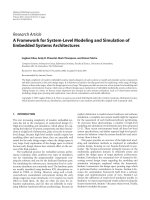
lated with authentic PEG standards (Figure 12.3 ). Figure 12.4 shows HPLC pro-
fi les of PEG before and after cultivation of microbial consortium E - 1 based on the
HPLC outputs and the PEG standards.

12.3.4
Numerical Study of Exogenous Depolymerization
Mathematical model (12.1) is appropriate for the depolymerization processes
under a steady microbial population. However, the change of microbial population
should be taken into account over a period in which a microbial population is still
in a developing stage. In such cases, the degradation rate should be time depend-
ent in the modeling of exogenous depolymerization processes:

d
d
x
t
tMx tM L
M
ML
y=− + +
+
ββ
(, ) (, )
(12.6)

Figure 12.2
HPLC outputs of PEG before and after the cultivation of the microbial consortium
E - 1.
mv/10
400
300
200
100
0

10 20
Min
30
DAY 0
DAY 1
DAY 3
DAY 5
DAY 7
DAY 9
12.3 Materials and Methods
289

Figure 12.3
PEG standards.
5
4
3
2
1
12 13 14 15 16 17 18 19 20 21 22
Logarithm of molecular weight
Retention time (min)
PEG STANDARDS
LEAST SQUARES APPROX

Figure 12.4
HPLC profi les of PEG before and after the cultivation of the microbial consortium
E - 1 [11, 12] .
0.03
0.02

Composition (%)
0.01
0.0
3.2
3.3 3.4 3.5 3.6 3.7 3.8 3.9 4.0 4.1 4.2
log M
BEFORE CULTIVATION
AFTER 1 DAY CULTIVATION
AFTER 3 DAY CULTIVATION
AFTER 5 DAY CULTIVATION
AFTER 7 DAY CULTIVATION
AFTER 9 DAY CULTIVATION

290
12 Modeling and Simulation of Microbial Depolymerization Processes of Xenobiotic Polymers
Solution
xwtM= (, )
of (12.6) is associated with the initial condition (12.2). Given
the degradation rate
β
(, )tM
, Eq. (12.6) and the initial condition (12.2) form an
initial value problem.
Time factors of the degradation rate such as microbial population, dissolved
oxygen, or temperature affect molecules regardless of their sizes. The dependence
of degradation rate on those factors is uniform over all molecules, and the degra-
dation rate should be a product of a time - dependent part
σ
()t
and a molecular

dependent part
λ
()M

βσλ
(, ) () ( )tM t M=
(12.7)
Note that
σ
()t
and
λ
()M
represent the magnitude and the molecular dependence
of degradability, respectively.
In order to simplify the model, let

τσ
=
∫
()ss
t
d
0
(12.8)
and

WM wtM XWM YWML(, ) (, ) (, ) (, )
τττ
== =+,,

Then

d
d
d
d
d
d
d
d
Xx
t
t
t
x
t
ττσ
==
1
()

and the exogenous depolymerization model (12.6) is converted into the equation

dX
d
Mx M L
M
ML
Y

τ
λλ
=−
()
++
+
()
(12.9)
This equation governs the transition of weight distribution
wM(, )
τ
under the time -
independent or time - averaged degradation rate
λ
()M
. Given the initial weight
distribution
fM()
, Eq. (12.9) forms an initial value problem together with the
initial condition

WM fM(, ) ( )0 =
(12.10)
Given an additional condition at
τ
=Τ
, Eq. (12.9) forms an inverse problem
together with the initial condition (12.10) and the fi nal condition (12.11), for which
the solution of the initial value problems (12.9) and (12.10) also satisfi es the fi nal
condition

WMgM(, ) ( )Τ= .
(12.11)
12.3 Materials and Methods
291
When the solution
W( , )
τ
M
of the initial value problem (12.9), (12.10) satisfi es the
condition (12.11), solution
wtM(, )
of the initial value problems (12.6) and (12.2)
satisfi es the condition (12.3), where

Τ=
∫
σ
()ss
T
d
0
(12.12)
Note that the inverse problem consisting of (12.9) – (12.11) is essentially identical
to the inverse problems (12.1) – (12.3). Numerical techniques developed for the
latter was applied to the former to fi nd the degradation rate
λ
()M
based on the
weight distribution before and after cultivation for 3 days [12, 13] (Figure 12.5 ).

12.3.5
Time Factor of Degradation Rate
A microbial population grows exponentially in a developing stage, and the increase
of biodegradability results from increase of microbial population. It is appropriate
to assume that the time factor of the degradation rate
σ
()t
is an exponential func-
tion of time

σ
()te
at b
=
+
(12.13)
In view of Eq. (12.8)

Figure 12.5
Degradation rate based on the weight distribution of PEG before and after the
cultivation of the microbial consortium E - 1 for 3 days [11, 12] .
140
PEG DEGRADATION RATE
130
120
110
100
90
80
70

60
50
40
30
20
10
0
3.2 3.3 3.4
Degradation rate (day)
log M
3.5 3.6 3.7 3.8 3.9 4.0 4.1 4.2

292
12 Modeling and Simulation of Microbial Depolymerization Processes of Xenobiotic Polymers

τσ
===−
∫∫
+
() ( )ss e s
e
a
e
t
as b
t
b
at
dd
00

1
(12.14)
It has been shown that the parameters
a
and
b
are uniquely determined provided
the weight distribution is given at
tT=
1
and
tT=
2
, where
0
12
<<TT
, and let

Τ
1
0
1
=
∫
σ
()ss
T
d
(12.15)

Τ
2
0
2
=
∫
σ
()ss
T
d
(12.16)
The condition (12.15) leads to

σ
()tee
ae
e
bat
at
aT
==
−
Τ
1
1
1
(12.17)
Now in view of (12.14),

τ
=
−
−
Τ
1
1
e
e
at
aT
1
1
(12.18)
Equation (12.16) leads to

ΤΤ
21
2
1
1
1
=
−
−

e
e
aT
aT

which is equivalent to the equation

ha()= 0
(12.19)
where

ha
e
e
aT
aT
()=
−
−
−
2
1
1
1
2
1
Τ
Τ

It has been shown that the condition

T
T
2

1
2
1
<
Τ
Τ
(12.20)
is a necessary and suffi cient condition for Eq. (12.19) to have a unique positive
solution [11] .
In order to determine
a
and
b
, let
T
11
3==Τ
. The initial value problems (12.9)
and (12.10) were solved numerically with the degradation rate shown in Figure
12.5 to reach the weight distribution at
τ
= 30
(Figure 12.6 ). Note that Figure 12.6