chemical kinetics with mathcad and maple
Bạn đang xem bản rút gọn của tài liệu. Xem và tải ngay bản đầy đủ của tài liệu tại đây (13.43 MB, 357 trang )
.
Viktor I. Korobov
l
Valery F. Ochkov
Chemical Kinetics with
Mathcad and Maple
SpringerWienNewYork
Ph.D. Viktor I. Korobov
Dnipropetrovsk National University
Department of Physical and Inorganic
Chemistry
Gagarin Avenue 72
49050 Dnipropetrovsk
Ukraine
/>Professor Valery F. Ochkov
Moscow Power Engineering Institute (TU)
Krasnokazarmennaya st. 14
Moscow
Russia
/>htm
This work is subject to copyright.
All rights are reserved, whether the whole or part of the material is concerned, specifically those
of translation, reprinting, re-use of illustrations, broadcasting, reproduction by photocopying
machines or similar means, and storage in data banks.
Product Liability: The publisher can give no guarantee for all the information contained in
this book. The use of registered names, trademarks, etc. in this publication does not imply,
even in the absence of a specific statement, that such names are exempt from the relevant
protective laws and regulations and therefore free for general use.
# 2011 Springer-Verlag/Wien
Printed in Germany
SpringerWienNewYork is a part of Springer Science+Business Media
springer.at
Cover design: WMXDesign GmbH, Heidelberg, Germany
Typesetting: SPi, Pondicherry, India
Printed on acid-free and chlorine-free bleached paper
SPIN: 80029760
Library of Congress Control Number: 2011928800
ISBN 978-3-7091-0530-6 e-ISBN 978-3-7091-0531-3
DOI 10.1007/978-3-7091-0531-3
SpringerWienNewYork
Preface
Chemical kinetics is one of the parts of physical chemistry with the most developed
mathematical description. Studying basics of chemical kinetics and successful
practical application of knowledge obtained demand proficiency in mathematical
formalization of certain problems on kinetics and making rather sophisticated
calculations. In this respect, it is difficult or sometimes even impossible to make
considerable part of such calculation without using a computer. With a mass of
literature on chemical kinetics the problems of practical computing the kinetics are
not actually discussed. For this reason the authors consider useful to state basics of
the formal kinetics of chemical reactions and approaches to two main kinetic
problems, direct and inverse, in terms of up-to-date mathematical packages
Maple and Mathcad.
Why did the authors choose these packages?
The history of using computers for scientific and technical calculation can be
conveniently divided into three stages:
l
Work with absolute codes
l
Programming using high-level languages
l
Using mathematical packages such as Mathcad, Maple, Matlab,
1
Mathematica,
MuPAD, Derive, Statistica, etc.
There are no clear boundaries between listed stages (information technologies).
Working in mathematical program one may insert an Excel table,
2
as the need
arose, or some user functions written in C language, which codes contain fragments
of assembler. Besides, absolute codes are still using in calculators, which are of
great utility in scientific and technical calculations. It is better to consider here not
isolated stages of computer technique development but a range of workbenches that
expand and interweave. This tendency results in sharp decrease of time required for
creating calculation methods and mathematical models, leads to refusal of a
1
Matlab is more likely a special programming language rather than a mathematical package.
2
The list of packages does not include Excel tables that are still the most popular application for
computing. However, Excel just as Matlab holds the half-way position between programming
languages and mathematical packages.
v
programmer as an additional link between a researcher and a computer, to openness
of calculations, enable us to see not only result, but all formulas in traditional
notation and also all intermediate data reinforced by plots and diagrams. It is
openness, clearness of Mathcad calculations that makes the package attractive
calculation and effective educational tool enabling us to use it as visualization of
the basics of chemical kinetics.
Maple is justly considered to be the best package of the symbolic mathematics,
particularly for analytical solution of differential equations. With this, the problems
on chemical kinetics are often resolved into this task.
Mathcad and Maple were developed as program applications alternative to
traditional programmin g languages. Sometimes a student or even a professional
cannot solve a chemical problem because a certain step transforms it from chemis-
try into informatics demanding deep knowledge of programming languages. How-
ever, as a rule a chemist has no such knowledge (and does not have to). Mathcad
and Maple enable us to solve a wide range of scientific, engineering, technical and
training problems without using traditional programming.
A reader getting acquainted with the book content may form an opinion that the
authors gave a slant towards Mathcad package and its “server development”, Math-
cad Application/Calculation Server. The case is that Mathcad was initially developed
as a tool for numerical calculations. In fact, numerical calculations lie at the center of
the book. At the same time, chemical kinetics also requires analytical,symbolic
calculations. If symbolic tools of Mathcad become insufficient for solving a particular
problem we decided to take advantages of Maple – an acknowledged leader among
systems of computer mathematics designed for analytical calculations.
Mathcad and Maple possess some properties allowing them to be popular both
among “non-programmers” and even among aces of programming. The point is that
work with these packages accelerates several times (in order) statement and solving
a problem. The similar situation occurred during conversion from absolute codes to
high-level programming languages (FORTRAN, Pascal, BASIC, etc.).
Even if a user knows programming languages quite well it is often appear helpful
to use Mathcad on a stage of formulat ion and debugging of a mathematical model.
One of the authors leads a team of programmers and engineers that has developed
and successfully markets WaterSteamPro program package ()
designed for calculations of thermal physical properties of the heat carriers at power
stations. The final version of the package was written and compiled on Visual C++,
but this project was hardly implemented without previous analysis of its formulae
and algorithms in Mathcad, which possesses convenient visualization tools for
numbers and formul ae.
It should be also noted that in distinction from Excel Mathcad enables us to
create calculations open for studying and further improvements.
“There is no rose without a thorn”. The main limitation of the mathematical
packages was that, as a rule, they couldn’t generate executable files (exe files),
which could be launched without the original program. In particular, this prevented
a progressive phenomenon - dividing those sitting in front of a screen into users
and developers. Usually, specialists working with mathematical programs, with
vi Preface
Mathcad, kept “subsistence production”: developed calculations for their own or for
the a few colleagues, who can work with Mathcad. They could give their results
only to those who had installed corresponding package. However, this person may
not buy a ready-made file but try to create required file by his own. Actually, we
consider now small calculations, which creating and checking out require time is
comparable with time for searching, installing, and learning the same ready – made
version. Although, rather bulky calculations find difficulty in opening the way to the
market: the personal calculation can be improved or enlarged at any time but in case
of somebody else’s calculation it is not. Here we can draw an analogy with another
“internal Mathcad” problem. Sometimes it is easier to create a user function than
find its completed version in the wilds of built-in Mathcad functions.
If a user was not acquainted with Mathcad package and did not have it in a
computer it was possible to give him (her) a file only with a significa nt load, on
condition that he (she) would install corresponding Mathcad version and would
learn at least the basics of the program. Often it required to upgrade both oper-
ating system and hardware, or even to buy a new computer. It was also necessary
to learn Mathcad.
Mathsoft Engineering and Education Inc., which was bought by PTC (http://
www.ptc.com), a new owner of Mathcad package, in 2006, took actions to improve
the situation. Firstly, they try to launch a free and shorten version, Mathcad
Explorer, together with the eighth Mathcad release. Mathcad Explorer enabled us
to open Mathcad files and calculate by them but not edit and save the documents on
disks. The program itself could be down loaded from the internet free of charge.
Secondly, the company actively developed tools for publication Mathcad work-
sheets on local networks and on the internet for studying but not for calculating.
One of the main consumers of the mathemat ical programs is education branch in
which the way to result, studying of the calculation methods, is more important than
the result itself. In particular, Mathcad 2001i version, in which the letter “i” meant
interactive, was designed for this.
However, all these solutions had no distant future. As was noted above, Mathcad
Explorer, a rather bulky program, should be downloaded from the network and
installed into a computer. In this case for solving intricate problems it is better to
install Mathcad itself, which is recently possible to download from the network for
prior charge, rather than a shorten version. On the other hand, it is desirable not only
to view Mathcad worksheets, or rather their html or MathML copies (casts), opened
on the network but also to transform them, change initial data and view (print, save)
a new result. The solution of this problem, almost complete rather than partial,
turned out to be possible with the help of internet again.
Mathcad Application Server (MAS) was put into operation in 2003 (it was
renamed into Mathcad Calcul ation Server – MA/CS in 2006) enabling us to run
Mathcad worksheets and call them remotely via the internet.
MA/CS technology allows us to solve the following problems:
l
There is no need to install required version of Mathcad, or it’s shorten version
Mathcad Explorer (see above), find somewhere, check executable files for
Preface vii
viruses and run them. We only have to connect computers to the Internet, access
MA/CS server using Internet Explorer (version 5.5 and higher) or any browser
installed in the palmtop computers or smart phones. This looks as if we work
with Mathcad worksheet: we can change source data; make calculation and get a
result (save and print). Calculation method (formulas in traditional notation but
not in the program form; this feature mak es Mathcad widespread) and interme-
diate data can be visible or hidden partially or completely.
l
New methods of calculation, open for studying, become available instantly to all
surfers of the Internet, or staff of a corporation, or researchers of a university. We
should only give corresponding addresses to users. Moreover, information about
suchlike calculations can appea r in the databases of different search engines
(yandex, google).
l
Any error, misprint, imperfection and assumption in a calculation noted by an author
or users can be corrected quickly. It is also easy to upgrade and extend calculations.
l
The MA/CS technology does not exclude tradition capability to download
Mathcad websheets from a server for their upgrading or extending. We only
should make a corresponding reference in a document. There are two ways of
using mcd-files. We can transfer them only for calculations on a working station
having Mathcad installed and lock documents with passwords. Another way is to
give them freely or sell them for work without limitations.
l
The MAS technology allows us to cut down expenses for mathematical software
for a corporation or a university. There is no need to install Mathcad to every
computer for routine calculations, to equip all computer classrooms. Mathcad
package is required now only for those who develop methods of calculations.
The others can use corporation (university or open to public) MA/CS.
It was MA/CS technology that used by the authors to develop educational project
on chemical kinetics: B/ChemKin.html. It is possi ble to
get access to Mathcad web sheets collection by this reference and make basic
kinetic calculations in remote access mode. For this purpose a user does to have
to install Mathcad on the computer.
This book was published in Russian in 2009. Due to the internet project on
chemical kinetics noted above almost all its pages have been translated into
English, and the book became familiar to a large number of chemists all over the
word. It becomes necessary to translate the book into English and supplem ent it
with new data that have been done by the authors.
The authors would like to acknowledge their colleagues and former students
who assisted in publication of the book:
Anna Grynova, Australian National University.
Natalia Yurchenko, Dnipropetrovsk National University.
Julia Chudova, Moscow Power Engineering Institute.
Alexander Zhurakovski, Oxford University.
Sasha Gurke, Knovel Corp.
Dnipropetrovsk, Ukraine Viktor I. Korobov
Moscow, Russia Valery F. Ochkov
viii Preface
Contents
1 Formally-Kinetic Description of One- and Two-Step Reactions 1
1.1 Main Concepts of Chemical Kinetics 1
1.2 Kinetics of Simple Reactions 4
1.3 Reactions, Which Include Two Elementary Steps 11
1.3.1 Reversible (Tw o-Way) Reactions 12
1.3.2 Consecutive Reactions 15
1.3.3 Parallel Reactions 27
1.3.4 Simplest Self-Catalyzed Reaction 31
2 Multi-Step Reactions: The Methods for Analytical Solving
the Direct Problem 35
2.1 Developing a Mathematical Model of a Reaction 35
2.2 The Classical Matrix Method for Solving the Direct Kinetic
Problem 41
2.3 The Laplace Transform in Kinetic Calculations 45
2.3.1 Brief Notes from Operational Calculus 45
2.3.2 Derivation of Kinetic Equations for Linear Sequences
of First-Order Reactions 48
2.3.3 Transient Regime in a System of Flow Reactors 53
2.3.4 Kinetic Models in the Fo rm of Equations Containing
Piecewise Continuous Functions 58
2.4 Approximate Methods of Chemical Kinet ics 59
2.4.1 The Steady-State Concentration Method 59
2.4.2 The Quasi-Equilibrium Approximation: Enzymatic
Reaction Kinetics 68
3 Numerical Solution of the Direct Problem in Chemical Kinetics 73
3.1 Given/Odesolve Solver in Mathcad System 73
3.1.1 Built-In Mathcad Integrators 79
ix
3.1.2 The Maple System Commands dsolve, odeplot
in Numerical Calculations 85
3.1.3 Oscillation Proce sses Modeling 87
3.1.4 Some Points on Non-Isothermal Kinetics 105
4 Inverse Chemical Kinetics Problem 115
4.1 Features of the Inverse Problem 115
4.2 Determination of Kinetic Parameters Using Data Linearization 117
4.2.1 Hydrolysis of Methyl Acetate in Acidic Media 117
4.2.2 Butadiene Dimerization: Finding the Reaction Order
and the Rate Constant 120
4.2.3 Exclusion of Time as an Independent Variable 123
4.2.4 Linearization with Numerical Integration of Kinetic
Data: Basic Hydrolysis of Diethyl Adipate 125
4.2.5 Estimation of Confidence Intervals for the Calculated
Constants 126
4.2.6 Kinetics of a-Pinene Isomerization 128
4.3 Inverse Problem and Special ized Minimization Methods 132
4.3.1 Deriving Parameters for an Empirical Rate Equation
of Phosgene Synthesis 133
4.3.2 Kinetics of Stepwise Ligand Exchange in Chrome
Complexes 137
4.3.3 Computing Kinetic Parameters Using Non-Linear
Approximation Tools 141
4.4 Universal Approaches to Inverse Chemical Kinetics Problem 148
4.4.1 Reversible Reaction with Dimerization of an Intermediate 148
5 Introduction into Electrochemical Kinetics 157
5.1 General Features of Electrode Processes 157
5.2 Kinetics of the Slow Discharge-Ionization Step 160
5.3 Electrochemical Reactions with Stepwise Electron Transfer 163
5.4 Electrode Processes Under Slow Diffusion Conditions 166
5.4.1 Relationship Between Rate and Potential Under
Stationary Diffusi on 168
5.4.2 Nonstationary Diffusion to a Spherical Electrode Under
Potentiostatic Conditions 174
5.5 Solution of a Problem of Nonstationary Spherical Diffusion
Under Potentiostatic Conditions 175
5.5.1 Nonstationary Diffusion Under Galvanostatic Conditions 179
6 Interface of Mathcad 15 and Mathcad Prime 183
6.1 Input/Displaying of Data 183
6.2 VFO (Variable-Function-Operator) 214
6.2.1 Function and Operator 214
x Contents
6.2.2 Variable Name 223
6.2.3 Invisible Variable 228
6.3 Comments in Mathcad Worksheets 235
6.4 Calculation with Physical Quantities: Problems and Solutions 240
6.5 Three Dimensions of Mathcad Worksheets . . . 253
6.6 Mathcad Plots 257
6.7 Animation and Pseudo-Animation 269
6.8 Mathcad Application Server 273
6.8.1 Continuation of Preface 273
6.8.2 Preparation of Mathcad Worksheet for Publicati on
Online or from WorkSheet to WebSheet 276
6.8.3 Web Controls: The Network Elements of the Interface 277
6.8.4 Comments in the WebSheets 295
6.8.5 Inserting Other Applications 297
6.8.6 Names of Variables and Functions 298
6.8.7 Problem of Extensional Source Data . 299
6.8.8 Knowledge Checking Via MAS 301
6.8.9 Access to Calculations Via Password . . 303
7 Problems 309
Bibliography 339
About the Authors 341
Index 343
Contents xi
.
Chapter 1
Formally-Kinetic Description
of One- and Two-Step Reactions
1.1 Main Concepts of Chemical Kinetics
We must accept that in order to describe the chemical system it is urgent for us to
know the exact way it follows during the transformation of the reag ents into the
products of the reaction. Knowledge of that kind gives us a possibility to command
chemical transformation deliberately. In other words, we need to know the mecha-
nism of the chemical transformation. Time evolution of the transition of the
reactionary system from the unconfigured state (parent materials) to the finite
state (products of the reaction) is of great importance too, because it is information
of how fast the reaction goes. Chemical kinetics is a self-contained branch of
chemical knowledge, which investigates the mechanisms of the reactions and the
patterns of their passing in time, and which gives us the answers to questions from
above.
Chemical kinetics together with chemical thermodynamics forms two corner
stones of the chemical knowledge. However, classic thermodynamic approach to
the description of the chemical systems is based on the consideration of the
unconfigured and finite states of the system exceptionally, with the absolute
abstracting from any assumptions about the methods (ways) of the transition of
the system from the unconfigured to the finite state. Thermodynamics can define
whether the system is in equilibrium state. If it is not, than thermodynamics states
that the system would certainly pass into the equilibrium state, because the factors
for such transition exist. Still, it is impossible to predict, what the dynamics of such
transition would be, that is in what time the equilibrium state will come, in terms of
classic thermodynam ic approaches. Such problems are not in interest of thermody-
namics, and the time coordinate is absolutely extraneous to the thermodynamics
approach. This is the distinction of kind between thermodynamic and kinetic
methods of the description of the chem ical systems.
The mainframe notion of the chemical kinetics is the rate of the reaction.
Reaction rate is defined as the change in the quantity of the reagent in time unit,
referred to the unit of the reactionary space. The concept of reactionary space
differs depending on the nature of the reaction. In the homogeneous system the
V.I. Korobov and V.F. Ochkov, Chemical Kinetics with Mathcad and Maple,
DOI 10.1007/978-3-7091-0531-3_1,
#
Springer-Verlag/Wien 2011
1
reaction is carried out in the whole volume, whereas in the heterogeneous system –
at the phase interface. In mathematic terms:
r ¼Æ
dn
Vdt
ðhomogeneous reactionÞ;
r ¼Æ
dn
Sdt
ðheterogeneous reactionÞ:
Derivative’s side here formally shows if the current substanc e is accumulated or
consumed during the reaction. If the volume of the system in the homogeneous
reaction is constant (closed system), then dn/V ¼ dC, and therefore, the rate is
interrelated to the change of the molar concentration of the reagent in time:
r ¼Æ
dC
dt
:
The change of the concentrations of the substances is different due to the
different stoichiometry of the interaction between them; therefore more exact
expression for the rate is as following:
r ¼ n
À1
i
dC
i
dt
;
where v
i
is a stoichiometric coefficient of the i participant of the reaction. For
example, for reaction:
aA þbB ! cC þ dD;
r ¼À
1
a
dC
A
ðtÞ
dt
¼À
1
b
dC
B
ðtÞ
dt
¼
1
c
dC
C
ðtÞ
dt
¼
1
d
dC
D
ðtÞ
dt
:
It is considered that the reaction rate is a positive magnitude; therefore the
stoichiometric coefficients of parent substances are taken with negative side.
The mathematic basis for the quantitative description of the reaction is the
fundamental postulate of the chemical kinetics – the law of mass action. In kinetic
formulation this law expresses the proportionality between the rate and the con-
centrations of the reagents:
r ¼ k
Y
i
c
i
n
i
:
Here k –isarate constant. It is a major kinetic parameter, which formally
expresses the value of the rate when the concentrations of the reagents equal to one.
The rate const ant does not depend on the concentrations of the substances and on
2 1 Formally-Kinetic Description of One- and Two-Step Reactions
time, but for most reactions it depends on the temperature. The exponent of
concentrations n is called a reaction order for i substance. To understand this
notion we need to define simple and complex reaction.
It is assumed in the formal kinetics that if the transition of the unconfigured
reagents into the products is not accompanied by the formation of intermediates of
any kind, i.e., goes in one stage, and then such reaction is simple or elementary. For
example, if it is known, that reaction
A þ2B ! Products;
is simple, then the equation for the law of mass action for it would be:
r ¼ kC
A
ðtÞ
1
C
B
ðtÞ
2
:
In this case the reaction orders for each substance are exactly equal to their
stoichiometric coefficients. In this case one says, that reaction has first order for
substance A and second order for substance B. The sum of the reaction orders for
each substance gives a common reaction order. It is obvious then, that given
example is a reaction of third order.
If the process of chemical transformation goes in more than one stage, than such
reaction is complex. Generally for complex reaction there is inconsistency between
stoichiometric and kinetic equations. In the equation for the law of mass action for
the complex reaction the exponents of the concentrations are some numbers,
defined experimentally, and in most cases are not equal to the stoichiometric
coefficients.
There are direct and inverse problems of chemical kinetics.
Starting point for solution of the direct problem of chemical kinetics is a kinetic
scheme of the reaction, which reflects assumed mechanism of the chemical trans-
formation. The mechanism in terms of formal kinetics is a certain totality of the
elementary stages (elementary reactions), through which a transformation of the
unconfigured substances into the finite products goes. Furthermore a mathematic
model of the reaction is formed on the basis of the postulate scheme. From the
definition of the reaction rate as a time derivative of the concentration of the reagent
it follows, that for the N participants of a multi-stage reaction its mathematic model
is a set of N differential equations, with each of them describing the rate of expense
or accumulation of each participant of the reaction. Time dependences of concen-
trations, obtained in the result of the equations set solution, are so called kinetic
curves. Analytic solution gives a set of equations of kinetic curves in the integrated
form, numerical – a set of concentrations of the substances in certain moments
of time.
In the inverse problem of chemical kinetics kinetic parameters of the reaction
(reaction orders for reagents, rate constants) are calculated using experimental data.
The goal of the inverse problem is to reconstruct of the kinetic scheme of the
transformations, i.e., to define the mechanism of the reaction.
1.1 Main Concepts of Chemical Kinetics 3
1.2 Kinetics of Simple Reactions
Let us consider a direct kinetic problem for simple reaction s in the closed exother-
mic system (the volume and the temperature are constant). If we assume the
correspondence between kinetic and stoichiometric equations, the scheme of the
simple reaction with sole reagent going in one stage could be written as:
nAÀÀÀ!
k
Products,
where n is a reaction order, in this case has a value equal to the stoichiometric
coefficient. We can mark out the cases of mono-, bi- and three-molecular reactions
with only one reagent depending on the value of n. The mathematic model of such
reactions could be expressed by the differential equation
dC
A
ðtÞ
dt
¼ÀkC
A
ðtÞ
n
: (1.1)
with an initial condition, which corresponds to the concentration of reagent A at the
moment of the start of the reaction (t ¼ 0):
C
A
ð0Þ¼C
A
0
:
Concentration C
A
0
is called an initial concentration, and the values C
A
(t) in each
moment of time – the current concentrations. An analytic solution of the direct
kinetic problem is a definition of the functional connection between current con-
centration and time.
In (1.1) variabl es are separated, therefore its solution could be accomplished in
MathCAD (Fig. 1.1). Prior to the interpretation the results of the solution we need to
examine document in Fig. 1.1 in detail. In the strict sense MathCAD does not have
on-board sources for the analytic solution of the differential equations, therefore
given solution is obtained in a little artificial way. Firstly, the variables were
preliminarily separated, and the equation was represented in the form of equality,
whose both parts were completely prepared for the integration. Secondly, both parts
of the equation were written in such a way, that the names of the integration
variables differed from the names of the variables, used as the limits of integration.
However, we have obtained a solution of the direct kinetic problem, which allows
writing a time-dependence of the reagent’s current concentration:
k ¼
1
n À1ðÞt
1
C
A
nÀ1
À
1
C
A
0
nÀ1
: (1.2)
Evidently concentration of the reagent decreases in time differently depending
on the reaction order. Thus, if the reaction order is formally conferred to the values
of 0, 2 or 3, we will obtain:
4 1 Formally-Kinetic Description of One- and Two-Step Reactions
C
A
ðtÞ¼C
A
0
À kt ðzero orderÞ; (1.3)
C
A
ðtÞ¼
C
A
0
1 þkC
A
0
t
ðsecond orderÞ; (1.4)
C
A
ðtÞ¼
C
A
0
ffiffiffiffiffiffiffiffiffiffiffiffiffiffiffiffiffiffiffiffiffiffiffi
1 þ2kC
A
0
2
t
q
ðthird orderÞ: (1.5)
Apparently an equation in the form (1.2) is inapplicable to the first-order
reaction, since when n ¼ 1 it contains uncertainty of a type 0/0. However, uncer-
tainty could be expanded due to l’Hopital’s rule. Getting of the integrated form of
the kinetic equation by differentiation with respect to the variable n of the numera-
tor and the denominator for the (1.2) is shown in Fig. 1.2.
Thus in the first-order reaction current concentration decreases in time by the
exponential law:
C
A
ðtÞ¼C
A
0
e
Àkt
: (1.6)
Obtained dependences (1.3)–(1.6) are also called the equations of kinetic curves.
Kinetic curves themselves are properly represented with graphs. Thus kinetic
Fig. 1.1 Analytic solution of the direct kinetic problem for the simple reaction by the means of
Mathcad package
1.2 Kinetics of Simple Reactions 5
curves for the reagent in hypothetic reactions of different orders and same values of
rate constant and initial concentrations of the reagent are show n in Fig. 1.3. As seen
with the increase of the order the decrease in reagent’s concentration in time
becomes less intensive.
Examined case of simple reaction with sole reagent can be extended to some
reaction with few reagents. For example, let the kinetic scheme of the reaction is
A þB ÀÀÀ!
k
Products:
If initial concentrations of the reagents A and B are equal, i.e., C
A
0
¼ C
B
0
, then
due to the stoichiometry of the reaction:
C
A
ðtÞ¼C
A
0
À xðtÞ;
C
B
ðtÞ¼C
B
0
À xðtÞ:
Fig. 1.2 The derivation of the kinetic equation of the first-order reaction
Fig. 1.3 Kinetic curves of the reagent in the elementary reactions of various orders
6 1 Formally-Kinetic Description of One- and Two-Step Reactions
Same quantities of both reagents, equal to x moles, would have reacted in the
unit of volume b y the moment of time t. Hence, C
A
ðtÞ¼C
B
ðtÞ and
dC
A
ðtÞ
dt
¼ÀkC
A
ðtÞC
B
ðtÞ¼ÀkC
A
ðtÞ
2
:
Consequently, time-dependence of the reagent’s A concentration is described by
(1.4). In the same manner it could be shown that (1.5) is true for the description of
the simple reaction’s kinetics
A þB þC ÀÀÀ!
k
Products,
when the initial concentrations of all three reagents are equal.
Other versions of the transformations with the participation of several reagents
are also possible, and for them obtained kinetic equations are true too. Let us
assume, that there is an interactions by the scheme A þ B ! Products, but reagent
B is taken in such excess comparing to reagent A before the start of the reaction, that
the change of its concentration during the reaction could be neglected and we can
consider C
B
(t) ¼ const. Then
dC
A
ðtÞ
dt
¼ÀkC
A
ðtÞC
B
ðtÞ%k
0
C
A
ðtÞ:
In this case constant k
0
include practically unchan geable in time concentration of
the substance B and is called an effective rate constant unlike true rate const ant k.
The change of reagent’s A concentration corresponds to the patterns of the first-
order reaction (1.6). However in this case it is said that reaction has a pseudo-
first order.
Another important characteristic of the simple reaction is a half-life time t
1/2
–time
from the moment of the beginning of the reaction, during which half of the initial
quantity of the substance reacts:
C
A
ðtÞ
t¼t
1=2
¼ C
A
0
=2:
It is to determine the connection between the half-life time and the initial
reagent’s concentration on the basis of the integrated forms of the kinetic equations
of various orders (Fig. 1.4).
Due to Fig. 1.4, the character of this connection changes in principle with the
change of the reaction order. Thus, half-life time in the zero-order reaction is
directly proportional to the reagent’s initial concentration. Half-life time in the
first-order reaction is defined only by the value of the rate constant and does not
depend on C
A
0
. t
1/2
in the second-order reaction is inversely proportional to the
initial concentration of the reagent, and in the third-order reaction – to the square of
the reagent’s initial concentration. These kinds are used in practice to define the
order of the investigated reaction by the experimental data.
1.2 Kinetics of Simple Reactions 7
Kinetic equations of the reactions of various orders are often represented in the
linear form. Thus, (1.6) for the first-order reaction looks as following after taking
the logarithm:
ln C
A
ðtÞ¼ln C
A
0
À kt: (1.7)
Kinetic equations for the second- and third-order reactions could be expressed as
following:
1
C
A
ðtÞ
¼
1
C
A
0
þ kt ðsecond orderÞ; (1.8)
1
2C
A
ðtÞ
2
¼
1
2C
A
0
ðtÞ
2
þ kt ðthird orderÞ: (1.9)
It is follows from (1.7)–(1.9), that for the reaction of each order linearize
coordinates exist. These are the coord inates, in which kinetic curves could be
represented in the form of straight line. Thus, kinetic curve of the reagent in the
first-order reaction is linearized in the coordinates ln C
A
from t. For the second- and
Fig. 1.4 Half-life times for the reactions of various orders
8 1 Formally-Kinetic Description of One- and Two-Step Reactions
third-order reactions linearize coordinates are 1/C
A
from t and 1/C
A
2
from t corre-
spondingly. In the zero-order reaction, as it follows from (1.3), time-dependence of
the reagent’s current concentration is linear. Model kinetic curves for the reactions
of various orders and their anamorphosises in corresponding coordinates are given
in Fig. 1.5. There is a very important condition: the slopes of the obtained straight
lines are defined by the value of the rate constant. This fact gives us an opportunity
to define the rate constant on the basis of the experimental kinetic data (see
Chap. 4).
For the second-order reaction with two reagents that have different initial
concentration C
A
0
and C
B
0
, mathematical model is:
dxðtÞ
dt
¼ kC
A
0
À xðtÞðÞC
B
0
À xðtÞðÞ;
where x(t) is quantity of the reagent, that has had reacted by the moment of time
t (initial condition – x(0) ¼ 0). The solution of the direct kinetic problem could be
expressed as
xðtÞ¼C
A
0
C
B
0
e
C
A
0
ÀC
B
0
ðÞ
kt
À 1
C
A
0
e
C
A
0
ÀC
B
0
ðÞ
kt
À C
B
0
:
Fig. 1.5 Model kinetic curves for the reactions of various orders and their anamorphosises in
linearize coordinates
1.2 Kinetics of Simple Reactions 9
At that the kinetic curves of the separate reagents are defined by the ratios:
C
A
ðtÞ¼C
A
0
À xðtÞ;
C
B
ðtÞ¼C
B
0
À xðtÞ:
The integrated form o f the kinetic equation for this case could be also represe nted
in the form, which indicates the possibility of the linearization of the kinetic data:
kt ¼
1
C
A
0
À C
B
0
ln
C
B
0
C
A
0
À xðtÞ½
C
A
0
C
B
0
À xðtÞ½
:
Getting corresponding equations and the calculation of the kinetic curves by the
means of Mathcad is shown in Fig. 1.6 .
Now we discuss the questions of the kinetics of the reactions of various orders,
and in many respects we consider order as a formal value, and do not use the
specific examples of chemical transformations. Essentially, this is the very pecu-
liarity of the formal-kinetic approach to the description of the reactions. Reaction
Fig. 1.6 The solution of the direct kinetic problem for the second-order reaction in case of
inequality of the reagents’ initial concentrations (on-line calculation />Worksheets/Chem/ChemKin-1-06-MCS.xmcd)
10 1 Formally-Kinetic Description of One- and Two-Step Reactions
order is a value, which could not be calculated theoretically for the specific reaction,
it could only be defined on the basis of data, obtained from the chemical experi-
ment. Practice proves that the majority of the reactions have first or second order.
Third-order reactions are extremely uncommon. The conception of the collision of
two reacting particles in the reactionary medium is a very convenient visual
metaphor of the chemical interaction. If we imagine such collision as an elementary
act, leading to the appearance of the products of the reaction, then it becomes
obvious, that the probability of two particles meeting each other at some point of the
medium is much higher, then the probability of the collision between three parti-
cles. Because of this reason there is much more second-order reactions, then third-
order reactions. And we do not even take in an account the possibility of the
reactions of highe r orders.
From the other side, the knowledge of the individual reaction order says nothing
about its mechanism. For example, if we experimentally define the first kinetic
order of the reaction, it does not necessarily mean, that this reaction is simple.
Experimentally defined order can be a pseudo-order or it can indicate, that the
investigated reaction is complex, and the behavior of the system is defined by some
limitative stage, which has the same order as the one defined experimentally. We
can state unambiguously, that the presence of the fractional or negative order of the
reaction is the evidence of its complex mechanism. Some reactions have zero order.
This value of the order is typical either for complex or for simple reactions that
follow special mechanism, which provides such energetic conditions of the inter-
actions between reactionary particles, in which the rate of the reaction does not
depend on the concentration.
1.3 Reactions, Which Include Two Elementary Steps
A complex reaction includes more than one elementary stage. Formal-kinetic
description of the complex reactions is based upon the principle of the indepen-
dence of the reactions’ passing . The main point of this principle is that if some
reaction is a separate stage of a complex chemical transformation, then it goes
under the same kinetic rules, as if the other stages were absent. A consequent of that
principle is used in mathematic analysis: if there are several elementary stages with
the participation of the same substance, then the change of its concentration is an
algebraic sum of the rates of all those stages, multiplied by the stoichiometric
coefficient of this substance in each sta ge. In this case a stoichiometric coefficient is
taken with the positive sign, if in this particular stage the substance is formed, and
with the negative sign, if it is expended. Let us illustrate the essence of this principle
with the example of the interaction between the nitric (III) oxide and chlorine due to
the overall reaction:
2NO þCl
2
! 2NOCl:
1.3 Reactions, Which Include Two Elementary Steps 11
Reductive mechanism of this reaction could be expressed with the order of two
elementary stages:
NO þCl
2
ÀÀÀ!
k
1
NOCl
2
;
NOCl
2
þ NO ÀÀÀ!
k
2
2NOCl:
Full mathematic model of the process is a set of differential equations, which
describe the change of the concentration of each reaction participant in time. Let us
draw attention to the fact, that initial reagent NO and intermediate product NOCl
2
participate in both stages of the process. Due to the principle of the independence of
reactions’ passing
dC
NO
ðtÞ
dt
¼À1ðÞr
1
þÀ1ðÞr
2
¼Àr
1
Àr
2
¼Àk
1
C
NO
ðtÞC
Cl
2
ðtÞÀk
2
C
NOCl
2
ðtÞC
NO
ðtÞ;
dC
NOCl
2
ðtÞ
dt
¼þ1ðÞr
1
þÀ1ðÞr
2
¼ r
1
À r
2
¼ k
1
C
NO
ðtÞC
Cl
2
ðtÞÀk
2
C
NOCl
2
ðtÞC
NO
ðtÞ:
Let us examine the regularities of some complex reactions, consisting of two
elementary first-order stages. Such reactions could be expressed with following
transformation schemes:
A
ÀÀÀÀ!
ÀÀÀÀ
k
1
k
2
Bðreversible reactionÞ;
AÀÀÀ!
k
1
BÀÀÀ!
k
2
Cðsuccessive reactionÞ;
A
ÀÀÀÀ!
ÀÀÀÀ!
k
1
k
2
B
C
ðparallel reactionÞ:
1.3.1 Reversible (Two-Way) Reactions
In reversible reactions the transformation of reagent into product is complicated
by simultaneous reverse conversion. Due to the principle of independence of the
elementary stages passing the rate of the reversible reaction is defined by the
difference between rates of direct and reverse stages. Example for reaction
A
ÀÀÀÀ!
ÀÀÀÀ
k
1
k
2
B;
12 1 Formally-Kinetic Description of One- and Two-Step Reactions