computational methods for multiphase flow
Bạn đang xem bản rút gọn của tài liệu. Xem và tải ngay bản đầy đủ của tài liệu tại đây (5.43 MB, 484 trang )
This page intentionally left blank
COMPUTATIONAL METHODS FOR MULTIPHASE FLOW
Predicting the behavior of multiphase flows is a problem of immense im-
portance for both industrial and natural processes. Thanks to high-speed
computers and advanced algorithms, it is starting to be possible to simulate
such flows numerically. Researchers and students alike need to have a one-
stop account of the area, and this book is that: it’s a comprehensive and
self-contained graduate-level introduction to the computational modeling of
multiphase flows. Each chapter is written by a recognized expert in the field
and contains extensive references to current research. The books is orga-
nized so that the chapters are fairly independent, to enable it to be used for
a range of advanced courses. In the first part, a variety of different numer-
ical methods for direct numerical simulations are described and illustrated
with suitable examples. The second part is devoted to the numerical treat-
ment of higher-level, averaged-equations models. No other book offers the
simultaneous coverage of so many topics related to multiphase flow. It will
be welcomed by researchers and graduate students in engineering, physics,
and applied mathematics.
COMPUTATIONAL METHODS FOR
MULTIPHASE FLOW
Edited by
ANDREA PROSPERETTI AND GR
´
ETAR TRYGGVASON
CAMBRIDGE UNIVERSITY PRESS
Cambridge, New York, Melbourne, Madrid, Cape Town, Singapore, São Paulo
Cambridge University Press
The Edinburgh Building, Cambridge CB2 8RU, UK
First published in print format
ISBN-13 978-0-521-84764-3
ISBN-13 978-0-511-29454-9
© Cambridge University Press 2007
2006
Information on this title: www.cambridge.org/9780521847643
This publication is in copyright. Subject to statutory exception and to the provision of
relevant collective licensing agreements, no reproduction of any part may take place
without the written
p
ermission of Cambrid
g
e University Press.
ISBN-10 0-511-29454-9
ISBN-10 0-521-84764-8
Cambridge University Press has no responsibility for the persistence or accuracy of urls
for external or third-party internet websites referred to in this publication, and does not
g
uarantee that any content on such websites is, or will remain, accurate or a
pp
ro
p
riate.
Published in the United States of America by Cambridge University Press, New York
www.cambridge.org
hardback
eBook (EBL)
eBook (EBL)
hardback
Contents
Preface page vii
Acknowledgments x
1 Introduction: A computational approach to multiphase flow 1
A. Prosperetti and G. Tryggvason
2 Direct numerical simulations of finite Reynolds number flows 19
G. Tryggvason and S. Balachandar
3 Immersed boundary methods for fluid interfaces 37
G. Tryggvason, M. Sussman and M.Y. Hussaini
4 Structured grid methods for solid particles 78
S. Balachandar
5 Finite element methods for particulate flows 113
H. Hu
6 Lattice Boltzmann models for multiphase flows 157
S. Chen, X. He and L S. Luo
7 Boundary integral methods for Stokes flows 193
J. Blawzdziewicz
8 Averaged equations for multiphase flow 237
A. Prosperetti
9 Point-particle methods for disperse flows 282
K. Squires
10 Segregated methods for two-fluid models 320
A. Prosperetti, S. Sundaresan, S. Pannala and D.Z. Zhang
11 Coupled methods for multifluid models 386
A. Prosperetti
References 436
Index 466
v
Preface
Computation has made theory more relevant
This is a graduate-level textbook intended to serve as an introduction to
computational approaches which have proven useful for problems arising in
the broad area of multiphase flow. Each chapter contains references to the
current literature and to recent developments on each specific topic, but the
primary purpose of this work is to provide a solid basis on which to build
both applications and research. For this reason, while the reader is expected
to have had some exposure to graduate-level fluid mechanics and numerical
methods, no extensive knowledge of these subjects is assumed. The treat-
ment of each topic starts at a relatively elementary level and is developed
so as to enable the reader to understand the current literature.
A large number of topics fall under the generic label of “computational mul-
tiphase flow,” ranging from fully resolved simulations based on first prin-
ciples to approaches employing some sort of coarse-graining and averaged
equations. The book is ideally divided into two parts reflecting this distinc-
tion. The first part (Chapters 2–5) deals with methods for the solution of
the Navier–Stokes equations by finite difference and finite element methods,
while the second part (Chapters 9–11) deals with various reduced descrip-
tions, from point-particle models to two-fluid formulations and averaged
equations. The two parts are separated by three more specialized chap-
ters on the lattice Boltzmann method (Chapter 6), the boundary integral
method for Stokes flow (Chapter 7), and on averaging and the formulation
of averaged equation (Chapter 8).
This is a multi-author volume, but we have made an effort to unify the
notation and to include cross-referencing among the different chapters. Hope-
fully this feature avoids the need for a sequential reading of the chapters, pos-
sibly aside from some introductory material mostly presented in Chapter 1.
The objective of this work is to describe computational methods, rather
vii
viii Preface
than the physics of multiphase flow. With this aspect in mind, the primary
criterion in the selection of specific examples has been their usefulness to
illustrate the capabilities of an algorithm rather than the characteristics of
particular flows.
The original idea for this book was conceived when we chaired the Study
Group on Computational Physics in connection with the Workshop on Sci-
entific Issues in Multiphase Flow. The workshop, chaired by Prof. T.J.
Hanratty, was sponsored by the U.S. Department of Energy and held on the
campus of the University of Illinois at Urbana-Champaign on May 7–9 2002;
a summary of the findings has been published in the International Journal
of Multiphase Flow, Vol. 29, pp. 1041–1116 (2003). As we started to col-
lect material and to receive input form our colleagues, it became clearer
and clearer that multiphase flow computation has become an activity with
a major impact in industry and research. While efforts in this area go back
at least five decades, the great improvement in hardware and software of the
last few years has provided a significant impulse which, if anything, can be
expected to only gain momentum in the coming years.
Most multiphase flows inherently involve a multiplicity of both temporal
and spatial scales. Phenomena at the scale of single bubbles, drops, solid
particles, capillary waves, and pores determine the behavior of large chem-
ical reactors, energy production systems, oil extraction, and the global cli-
mate itself. Our ability to see how the integration across all these scales
comes about and what are its consequences is severely limited by this mind-
boggling complexity. This is yet another area where computing offers a
powerful tool for significant progress in our ability to understand and
predict.
Basic understanding is achieved not only through the simulation of actual
physical processes, but also with the aid of computational “experiments.”
Multiphase flows are notorious for the difficulties in setting up fully con-
trolled physical experiments. However, computationally, it is possible, for
example, to include or not include gravity, account for the effects of a well-
characterized surfactant, and others. It is now possible to routinely compute
the behavior of relatively simple systems, such as the breakup of jets and
the shape of bubbles. The next few years are likely to result in an explosion
of results for such relatively simple systems where computations will help
us gain a very complete picture of the relevant physics over a large range
of parameters. A strong impulse to these activities will be imparted by
effective computational methods for multiscale problems, which are rapidly
developing.
At a practical, industrial level, simulation must rely on an averaged
Preface ix
description and closure models to account for the unresolved phenomena.
The formulation of these closures will greatly benefit from the detailed sim-
ulation of the underlying microphysics. The situation is similar to single-
phase turbulent flows where, in the last two decades, simulations have played
a major role, e.g. in developing large-eddy models.
It is in the examination of very complex, very large-scale systems, where it
is necessary to follow the evolution of an enormous range of scales for a long
time, that the major challenges and opportunities lie. Such simulations, in
which it is possible to get access to the complete data and to control accu-
rately every aspect of the system, will not only revolutionize our predictive
capability, but also open up new opportunities for controlling the behavior
of such systems.
It is our firm belief that today we stand at the threshold of exciting develop-
ments in the understanding of multiphase flows for which computation will
prove an essential element. All of us – authors and editors – sincerely hope
that this book will contribute to further progress in this field.
Andrea Prosperetti
Gretar Tryggvason
Acknowledgments
The editors and the contributors to the present volume wish to acknowledge
the help and support received by several individuals and organizations in
connection with the preparation of this work.
• S. Balachandar’s research was supported by the ASCI Center for the
Simulation of Advanced Rockets at the University of Illinois at Urbana-
Champaign through the U.S. Department of Energy (subcontract number
B341494).
• Jerzy Blawzdziewicz would like to acknowledge the support provided
by NSF CAREER grant CTS-0348175.
• Howard H. Hu’s research was supported by NSF grant CTS-9873236
and by DARPA through a grant to the University of Pennsylvania.
• M. Yousuff Hussaini would like to acknowledge NSF contract DMS
0108672, and the support and encouragement of Provost Lawrence G.
Abele.
• Li-Shi Luo would like to acknowledge the support provided by NSF grant
CTS-0500213.
• Sreekanth Pannala and Sankaran Sundaresan would like thank
Tom O’Brien, Madhava Syamlal and the MFIX team. The contribution
has been partly authored by a contractor of the U.S. Government under
Contract No. DE-AC05-00OR22725. Accordingly, the U.S. Government
retains a non-exclusive, royalty-free license to publish or reproduce the
published form of this contribution, or allow others to do so, for U.S.
Government purposes.
• Andrea Prosperetti expresses his gratitude to Drs. Anthony
J. Baratta, Cesare Frepoli, Yao-Shin Hwang, Raad Issa, John H. Mahaffy,
Randi Moe, Christopher J. Murray, Fadel Moukalled, Sylvain Pigny,
x
Acknowledgments xi
Iztok Tiselj, and Vaughn E. Whisker. His work was supported by NSF
grant CTS-0210044 and by DOE grant DE-FG02-99ER14966.
• Mark Sussman’s contribution was supported in part by the National
Science Foundation under contract DMS 0108672
• Gretar Tryggvason would like to thank his graduate students and colla-
borators who have contributed to his work on multiphase flows. He would
also like to acknowledge support by DOE grant DE-FG02-03ER46083,
NSF grant CTS-0522581, as well as NASA projects NAG3-2535 and
NNC05GA26G, during the preparation of this book.
• Duan Z. Zhang would like to acknowledge many important discussions
and physical insights offered by Dr. F. H. Harlow. The Joint DoD/
DoE Munitions Technology Development Program provided the financial
support for this work.
1
Introduction: A computational approach to
multiphase flow
This book deals with multiphase flows, i.e. systems in which different fluid
phases, or fluid and solid phases, are simultaneously present. The fluids may
be different phases of the same substance, such as a liquid and its vapor, or
different substances, such as a liquid and a permanent gas, or two liquids.
In fluid–solid systems, the fluid may be a gas or a liquid, or gases, liquids,
and solids may all coexist in the flow domain.
Without further specification, nearly all of fluid mechanics would be in-
cluded in the previous paragraph. For example, a fluid flowing in a duct
would be an instance of a fluid–solid system. The age-old problem of the
fluid-dynamic force on a body (e.g. a leaf in the wind) would be another
such instance, while the action of wind on ocean waves would be a situation
involving a gas and a liquid.
In the sense in which the term is normally understood, however, multi-
phase flow denotes a subset of this very large class of problems. A pre-
cise definition is difficult to formulate as, often, whether a certain situation
should be considered as a multiphase flow problem depends more on the
point of view – or even the motivation – of the investigator than on its in-
trinsic nature. For example, wind waves would not fall under the purview of
multiphase flow, even though some of the physical processes responsible for
their behavior may be quite similar to those affecting gas–liquid stratified
flows, e.g. in a pipe – a prime example of a multiphase system. The wall of
a duct or a tree leaf may be considered as boundaries of the flow domain of
interest, which would not qualify these as multiphase flow problems. How-
ever, the flow in a network of ducts, or wind blowing through a tree canopy,
may be – and have been – studied as multiphase flow problems.
These examples point to a frequent feature of multiphase flow systems,
namely the complexity arising from the mutual interaction of many subsys-
tems. But – as a counterexample to the extent that it may be regarded as
1
2
‘simple’ – one may consider a single small bubble as an instance of multiphase
flow, particularly if the study focuses on features that would be relevant to
an assembly of such entities.
The interaction among many entities, such as bubbles, drops, or particles
immersed in the fluid, is not the only source of the complexity usually exhib-
ited by multiphase flow phenomena. There may be many other components
as well, such as the very physics of the problem (e.g. the advancing of a
solid–liquid–gas contact line, or the transition between different gas–liquid
flow regimes), the simultaneous occurring of phenomena spanning widely
different scales (e.g. oil recovery, where the flow at the single pore level
impacts the behavior of the entire reservoir), the presence of a disturbed
interface (e.g. surface waves on a falling film, or large, highly deformable
drops or bubbles), turbulence, and others.
This complexity strongly limits the usefulness of purely analytical meth-
ods. For example, even for the flow around bodies with a simple shape such
as spheres, most analytical results are limited to very small or very large
Reynolds numbers. The more common and interesting situation of inter-
mediate Reynolds numbers can hardly be studied by these means. When
two or more bodies interact, or the ambient flow is not simple, the power of
analytical methods is reduced further.
In a laboratory, it may even be difficult to set up a multiphase flow ex-
periment with the necessary degree of control: the breakup of a drop in a
turbulent flow or a precise characterization of the bubble or drop size dis-
tribution may be examples of such situations. Furthermore, many of the
experimental techniques developed for single-phase flow encounter severe
difficulties in their extension to multiphase systems. For example, even at
volume fractions of a few percent, a bubbly flow may be nearly opaque to op-
tical radiation so that visualization becomes problematic. The clustering of
suspended particles in a turbulent flow depends on small-scale details which
it may be very difficult to resolve. Little information about atomization can
be gained by local probes, while adequate seeding for visualization may be
impossible.
In this situation, numerical simulation becomes an essential tool for the
investigation of multiphase flow. In a limited number of cases, computa-
tion can solve actual practical problems which lend themselves to direct
numerical simulation (e.g. the flow in microfluidic devices), or for which suf-
ficiently reliable mathematical models exist. But, more frequently, compu-
tation is the only available tool to investigate crucial physical aspects of the
situation of interest, for example the role of gravity, or surface tension, which
can be set to arbitrary values unattainable with physical experimentation.
Multiphase Flow 3
Furthermore, the complexity of multiphase flows often requires reduced
descriptions, for example by means of averaged equations, and the formu-
lation of such reduced models can greatly benefit from the insight provided
by computational results.
The last decade has seen the development of powerful computational ca-
pabilities which have marked a turning point in multiphase flow research.
In the chapters that follow, we will give an overview of many of these devel-
opments on which future progress will undoubtedly be built.
1.1 Some typical multiphase flows
Having given up on the idea of providing a definition, we may illustrate the
scope of multiphase flow phenomena by means of some typical examples.
Here we encounter an embarrassment of riches. In technology, electric power
generation, sprays (e.g. in internal combustion engines), pipelines, catalytic
oil cracking, the aeration of water bodies, fluidized beds, and distillation
columns are all legitimate examples. As a matter of fact, it is estimated
that over half of anything which is produced in a modern industrial soci-
ety depends to some extent on a multiphase flow process. In Nature, one
may cite sandstorms, sediment transport, the “white water” produced by
breaking waves, geysers, volcanic eruptions, acquifiers, clouds, and rain. The
number of items in these lists can easily be made arbitrarily large, but it may
be more useful to consider with a minimum of detail a few representative
situations.
A typical example of a multiphase flow of major industrial interest is
a fluidized bed (see Section 10.4). Conceptually, this device consists of a
vertical vessel containing a bed of particles, which may range in size from
tens of microns to centimeters. A fluid (a liquid or, more frequently, a gas)
is pumped through the porous bottom of the vessel and through the bed. As
the flow velocity is increased, initially one observes an increasing pressure
drop across the bed. However, when the pressure drop reaches a value close
to the weight of the bed per unit area, the particles become suspended in the
fluid stream and the bed is said to be fluidized. These systems are useful
as they promote an intimate contact between the particles and the fluid
which facilitates, e.g., the combustion of material with a low caloric content
(such as low-grade coal, or even domestic garbage), the in situ absorption
of the pollutants deriving from the combustion (e.g. limestone particles
absorbing SO
2
), the action of a catalyst (e.g. in oil cracking), and others.
In order for the bed to fulfill these functions, it is desirable that it remain
homogeneous, which is exceedingly difficult to obtain. Indeed, under most
4
conditions, one observes large volumes of fluid, called bubbles, which contain
a much smaller concentration of particles than the average, and which rise
through the bed venting at its surface. In the regime commonly called
“channeling,” these particle-free fluid structures span the entire height of the
bed. It is evident that both bubbling and channeling reduce the effectiveness
of the system as they cause a large fraction of the fluid to leave the bed
contacting only a limited number of particles. The transition from the state
of uniform fluidization to the bubbling regime is thought to be the result
of an instability which is still incompletely understood after several decades
of study. The resulting uncertainty hampers both design tasks, such as
scale-up, and performance, by requiring operation with conservative safety
margins. Several different types of fluidized beds exist. Figure 1.1 shows
a diagram of a circulating fluidized bed, so called because the particles are
ejected from the top of the riser and then returned to the bed. The figure
illustrates the wide variety of situations encountered in this system: the
dense particle flow in the standpipe, the fast and dilute flow in the riser, the
balance between centrifugal and gravitational forces in the cyclones, and
wall effects.
It is evident that a system of this complexity is way beyond the reach of
direct numerical simulation. Indeed, the mathematical models in use rely
on averaged equations which, however, still suffer from several problems as
will be explained in Chapters 8 and 10. Attempts to improve these equa-
tions must rely on a good understanding of the flow through assemblies of
particles or, at the very least, of the flow around a particle suspended in a
fluid stream, possibly spatially non-uniform and temporally varying. Fur-
thermore, interactions with the walls are important. These considerations
are a powerful motivation for the development of numerical methods for the
detailed simulation of particle–fluid flow. Some methods suitable for this
purpose are described in Chapters 4 and 5 of this book.
An important natural phenomenon involving fluid–particle interactions is
sediment transport in rivers, coastal areas, and others. A significant differ-
ence with the case of fluidized beds is that, in this case, gravity tends to
act orthogonally to the mean flow. This circumstance greatly affects the
balance of forces on the particles, increasing the importance of lift. This
component of the hydrodynamic force on bodies of a general shape is still
insufficiently understood and, again, the computational methods described
in Chapters 2–5 are an effective tool for its investigation.
A bubble column is the gas–liquid analog of a fluidized bed. The bubbles
are introduced at the bottom of a liquid-filled column with the purpose of
increasing the interfacial area available for a gas–liquid chemical reaction,
Multiphase Flow 5
fluidizing
gas
gas
riser
aeration gas
standpipe
Fig. 1.1. This figure shows schematically one of several different configurations
of a circulating fluidized bed loop used in engineering practice. The particles flow
downward through the aerated “standpipe,” and enter the bottom of a fast fluidized
bed “riser.” The particles are centrifugally separated from the gas in a train of
“cyclones.” In this diagram, the particles separated in the primary cyclone are
returned to the standpipe while the fate of the particles removed from the secondary
cyclone is not shown.
of aerating the liquid, or even to lift the liquid upward in lieu of a pump.
Spatial inhomogeneities arise in systems of this type as well, and their effect
can be magnified by the occurrence of coalescence which may produce very
large gas bubbles occupying nearly the entire cross-section of the column and
separated by so-called liquid “slugs.” The transition from a bubbly to a slug-
flow regime is a typical phenomenon of gas–liquid flows, of great practical
importance but still poorly understood. Here, in addition to understanding
how the bubbles arrange themselves in space, it is necessary to model the
6
forces which cause coalescence and the coalescence process itself. These
are evidently major challenges in free-surface flows: Chapters 10 and 11
describe some computational methods capable of shedding light on such
phenomena.
Another system in which coalescence plays a major role is in clouds and
rain formation. Small water droplets fall very slowly and are easy prey to
the convective motions of the atmosphere. For rain to fall, the drops need to
grow to a sufficient size. Condensation is impeded by the slowness of vapor
diffusion through the air to reach the drop surface. The only possible expla-
nation of the observed short time scale for rain formation is the occurrence of
coalescence. Simple random collisions caused by turbulence are very unlikely
in dilute conditions. Rather, the process must rely on a subtler influence of
turbulence which can be studied with the aid of an approximation in which
the finite size of the droplets is (partially) disregarded. This approach to
the study of turbulence–particle interaction is a powerful one described in
Chapter 9. This is another example in which a critical ingredient to improve
modeling is a better understanding of fluctuating hydrodynamic forces on
particle assemblies which can only be gained by computational means.
Other important gas–liquid flows occur in pipelines. Here free gas may
exist because it is originally present at the inlet, as in many oil pipelines,
but it may also be due to the ex-solution of gases originally dissolved in
the liquid as the pressure along the pipeline falls. Depending on the liquid
and gas flow rates and on the slope of the pipeline, one may observe a
whole variety of flow regimes such as bubbly, stratified, wavy, slug, annular,
and others. Each one of them reacts differently to an imposed pressure
gradient. For example, in a stratified flow, a given pressure drop would
produce a much larger flow rate of the gas phase than of the liquid phase,
unlike a bubbly or slug-flow regime. In slug flow, solid surfaces such as
pumps and tube walls are often subjected to large fluctuating forces which
may cause dangerous vibration and fatigue. It is therefore of great practical
importance to be able to predict which flow regime would occur in a given
situation, the operational limits to remain in the desired regime, and how
the system would react to transients such as start-ups and shut-downs. The
experimental effort devoted to this subject has been very considerable, but
progress has proven to be frustratingly slow and elusive. The computational
methods described in Chapters 3, 10, and 11 are promising tools for a better
understanding of these problems.
Even remaining at the level of the momentum coupling between the phases,
all of the examples described so far are challenging enough that a com-
plete understanding is not yet available. When energy coupling becomes
Multiphase Flow 7
important, such as in combustion and boiling, the difficulties increase and,
with them, the prospect of progress by computational means. Boiling is
the premier process by which electric power is generated world-wide, and is
considered to be a vital means of heat removal in the computers of the future
and human activities in space. Yet, this is another instance of those pro-
cesses which have been very reluctant to yield their secrets in spite of nearly
a century of experimental and theoretical work. Vital questions such as
nucleation site density, bubble–bubble interaction, and critical heat flux are
still for the most part unanswered. For space applications, understanding
the role of gravity is an absolute prerequisite but microgravity experimen-
tation is costly and fraught with difficulties. Once again, computation is a
most attractive proposition. In this book, space constraints prevent us from
getting very far into the treatment of nonadiabatic multiphase flow. A very
brief treatment of energy coupling in the context of averaged equations is
presented in Chapter 11.
1.2 A guided tour
The book can be divided into two parts, arranged in order of increasing
complexity of the systems for which the methods described can be used.
The first part, consisting of Chapters 2–7, describes methods suitable for
the detailed solution of the Navier–Stokes equations for typical situations of
interest in multiphase flow. Chapter 8 introduces the concept of averaged
equations, and methods for their solution take up the second part of the
book, Chapters 9 to 11.
In Chapter 2 we introduce the idea of direct numerical simulation of mul-
tiphase flows, discussing the motivation behind such simulations and what
to expect from the results. We also give a brief overview of the various
numerical methods used for such simulations and present in some detail
elementary techniques for the solution of the Navier–Stokes equations. In
Chapter 3, numerical methods for fluid–fluid simulations are discussed. The
methods presented all rely on the use of a fixed Cartesian grid to solve the
fluid equations, but the phase boundary is tracked in different ways, using
either marker functions or connected marker particles. Computation of flows
over stationary solid particles is discussed in Chapter 4. We first give an
overview of methods based on the use of fixed Cartesian grids, along similar
lines as the methods presented in Chapter 3, and then move on to meth-
ods based on body-fitted grids. While less versatile, these latter methods
are capable of producing very accurate results for relatively high Reynolds
number, thus providing essentially exact solutions that form the basis for
8
the modeling of forces on single particles. Simulations of more complex
solid-particle flows are introduced in Chapter 5, where several versions of
finite element arbitrary Lagrangian–Eulerian methods, based on unstruc-
tured tetrahedron grids that adapt to the particles as they move, are used
to simulate several moving solid particles. One of the important applications
of simulations of this type may be in formulating closures of the averaged
quantities necessary for the modeling of multiphase flows in average terms.
Chapter 6 introduces the lattice Boltzman method for multiphase flows and
in Chapter 7 we discuss boundary integral methods for Stokes flows of two
immiscible fluids or solid particles in a viscous fluid. While restricted to a
somewhat special class of flows, boundary integral methods can reduce the
computational effort significantly and yield very accurate results.
Chapters 8–11 constitute the second part of the book and deal with sit-
uations for which the direct solution of the Navier–Stokes equations would
require excessive computational resources and the use of reduced descrip-
tions becomes necessary. The basis for these descriptions is some form of
averaging applied to the exact microscopic laws and, accordingly, the first
chapter of this group outlines the averaging procedure and illustrates how
the various reduced descriptions in the literature and in the later chap-
ters are rooted in it. A useful approximate treatment of disperse flows –
primarily particles suspended in a gas – is based on the use of point-particle
models, which are considered in Chapter 9. In these models, the fluid mo-
mentum equation is augmented by point forces which represent the effect of
the particles, while the particle trajectories are calculated in a Lagrangian
fashion by adopting simple parameterizations of the fluid-dynamic forces.
The fluid component of the model, therefore, looks very much like the ordi-
nary Navier–Stokes equations, and it can be treated by the same methods
developed for single-phase computational fluid dynamics. At present, this is
the only well-developed reduced-description approach capable of incorporat-
ing the direct numerical simulation of turbulence, and efforts are currently
under way to apply to it the ideas and methods of large-eddy simulation.
The point-particle model is only valid when the particle concentration is
so low that particle–particle interactions can be neglected, and the particles
are smaller than the smallest flow length scale, e.g. in turbulent flow, the
Kolmogorv scale. Therefore, while useful, the range of applicability of the
approach is rather limited. The following two chapters deal with models
based on a different philosophy of broader applicability, that of interpene-
trating continua. In the underlying conceptual picture it is supposed that
the various phases are simultaneously present in each volume element in
proportions which vary with time and position. Each phase is described by
Multiphase Flow 9
a continuity, momentum, and energy equation, all of which contain terms
describing the exchange of mass, momentum, and energy among the phases.
Numerically, models of this type pose special challenges due to the nearly
omnipresent instabilities of the equations, the constraint that the volume
fractions occupied by each phase necessarily lie between 0 and 1, and many
others.
In principle, the interpenetrating-continua modeling approach is very
broadly applicable to a large variety of situations. A model suitable for
one application, for example stratified flow in a pipeline, differs from that
applicable to a different one, for example, pneumatic transport, mostly in
the way in which the interphase interaction terms are specified. It turns
out that, for computational purposes, most of these specific models share a
very similar structure. A case in point is the vast majority of multiphase
flow models adopted in commercial codes. Two broad classes of numerical
methods are available. In the first one, referred to as the segregated approach
and described in Chapter 10, the various balance equations are solved se-
quentially in an iterative fashion starting from an equation for the pressure.
The general idea is derived from the well-known SIMPLE method of single-
phase computational fluid mechanics. The other class of methods, described
in Chapter 11, adopts a more coupled approach to the solution of the equa-
tions and is suitable for faster transients with stronger interactions among
the phases.
1.3 Governing equations and boundary conditions
In view of the prominent role played by the incompressible single-phase
Navier–Stokes equations throughout this book, it is useful to summarize
them here. It is assumed that the reader has a background in fluid mechan-
ics and, therefore, no attempt at a derivation or an in-depth discussion will
be made. Our main purpose is to set down the notation used in later chap-
ters and to remind the reader of some fundamental dimensionless quantities
which will be frequently encountered.
If ρ(x,t) and u(x,t) denote the fluid density and velocity fields at position
x and time t, the equation of continuity is
∂ρ
∂t
+ ∇∇
∇
· (ρu)=0. (1.1)
For incompressible flows this equation reduces to
∇∇
∇
· u =0. (1.2)
10
This latter equation embodies the fact that each fluid particle conserves its
volume as it moves in the flow.
In conservation form, the momentum equation is
∂
∂t
(ρu)+∇∇
∇
· (ρuu)=∇∇
∇
·σσ
σ
+ ρf, (1.3)
in which f is an external force per unit volume acting on the fluid. Very often,
the force f will be the acceleration of gravity g. However, as in Chapter 9,
one may think of very small suspended particles as exerting point forces
which can also be described by the field f. The stress tensor σσ
σ
may be
decomposed into a pressure p and viscous part ττ
τ
:
σσ
σ
= −pI + ττ
τ
, (1.4)
in which I is the identity two-tensor. In most of the applications that follow,
we will be dealing with Newtonian fluids, for which the viscous part of the
stress tensor is given by
ττ
τ
=2µe, e =
1
2
∇∇
∇
u + ∇∇
∇
u
T
, (1.5)
in which µ is the coefficient of (dynamic) viscosity, e the rate-of-strain tensor,
and the superscript T denotes the transpose; in component form:
e
ij
=
1
2
∂u
i
∂x
j
+
∂u
j
∂x
i
, (1.6)
in which x =(x
1
,x
2
,x
3
). With (1.5), (1.3) takes the familiar form of the
Navier–Stokes momentum equation for a Newtonian, constant-properties
fluid:
∂u
∂t
+ ∇∇
∇
· (uu)=−
1
ρ
∇∇
∇
p + ν∇∇
∇
2
u + f, (1.7)
in which ν = µ/ρ is the kinematic viscosity. Because of (1.2), this equation
may be written in non-conservation form as
∂u
∂t
+(u ·∇∇
∇
) u = −
1
ρ
∇∇
∇
p + ν∇
2
u + f, (1.8)
where the notation implies that the i-th component of the second term is
given by
[(u ·∇∇
∇
) u]
i
=
3
j=1
u
j
∂u
i
∂x
j
. (1.9)
When the force field f admits a potential U, f = −∇∇
∇
U, one may introduce
Multiphase Flow 11
the reduced or modified pressure, i.e. the pressure in excess of the hydrostatic
contribution,
p
r
= p + ρ U (1.10)
in terms of which (1.8) becomes
∂u
∂t
+(u ·∇∇
∇
) u = −
1
ρ
∇∇
∇
p
r
+ ν∇
2
u. (1.11)
In particular, for the gravitational force, U = −ρg ·x.
We have already noted at the beginning of this chapter that multiphase
flows are often characterized by the presence of interfaces. When there is a
mass flux ˙m across (part of) the boundary S separating two phases 1 and 2
as, for example, in the presence of phase change at a liquid–vapor interface,
conservation of mass requires that
˙m ≡ ρ
2
(u
2
− w) · n = ρ
1
(u
1
− w) · n (1.12)
where n is the unit normal and w · n the normal velocity of the interface
itself. An expression for this quantity is readily found if the interface is
represented as
S(x,t)=0. (1.13)
Indeed, at time t + dt, we will have S(x + wdt, t + dt) = 0 from which, after
a Taylor series expansion,
∂S
∂t
+ w ·∇∇
∇
S =0 on S =0. (1.14)
But the unit normal, directed from the region where S<0 to that where
S>0, is given by
n =
∇∇
∇
S
|∇∇
∇
S|
, (1.15)
so that
n ·w = −
1
|∇∇
∇
S|
∂S
∂t
. (1.16)
If S = 0 denotes an impermeable surface, as in the case of a solid wall, ˙m =0
so that n · u = n · w. In this case, by (1.12), (1.16) becomes the so-called
kinematic boundary condition:
∂S
∂t
+ u ·∇∇
∇
S =0 on S =0. (1.17)
At solid surfaces, for viscous flow, one usually imposes the no-slip condition,