convective heat transfer mathematical and computational modelling of viscous fluids and porous media
Bạn đang xem bản rút gọn của tài liệu. Xem và tải ngay bản đầy đủ của tài liệu tại đây (29.01 MB, 648 trang )
Convective Heat Transfer:
Mathematical and Computational Modelling of
Viscous Fluids and Porous Media
by Ioan I. Pop, Derek B. Ingham
• ISBN: 0080438784
• Pub. Date: February 2001
• Publisher: Elsevier Science & Technology Books
Preface
Interest in studying the phenomena of convective heat and mass transfer between
an ambient fluid and a body which is immersed in it stems both from fundamental
considerations, such as the development of better insights into the nature of the
underlying physical processes which take place, and from practical considerations,
such as the fact that these idealised configurations serve as a launching pad for
modelling the analogous transfer processes in more realistic physical systems. Such
idealised geometries also provide a test ground for checking the validity of theoretical
analyses. Consequently, an immense research effort has been expended in exploring
and understanding the convective heat and mass transfer processes between a fluid
and submerged objects of various shapes. Among several geometries which have
received considerable attention are flat plates, circular and elliptical cylinders and
spheres, although much information is also available for some other bodies, such as
corrugated surfaces or bodies of relatively complicated shapes.
It is readily recognised that a wealth of information is now available on con-
vective heat and mass transfer operations for viscous (Newtonian) fluids and for
fluid-saturated porous media under most general boundary conditions of practi-
cal interest. The number of excellent review articles, books and monographs, which
summarise the state-of-the-art of convective heat and mass transfer, which are avail-
able in in the literature testify to the considerable importance of this field to many
practical applications in modern industries.
Given the great practical importance and physical complexity of buoyancy flows,
they have been very actively investigated as part of the effort to fully understand,
calculate and use them in many engineering problems. No doubt, these flows have
been invaluable tools for the designers in a variety of engineering situations. How-
ever, it is well recognised that this has been possible only via appropriate heuristic
assumptions, see for example the Boussinesq (1903) and Prandtl (1904) boundary-
layer approximations. Today it is widely accepted that viscous effects, although very
often confined in small regions, control and regulate the basic features of the flow
and heat transfer characteristics, as for example, boundary-layer separation and flow
circulation. As a result, these characteristics depend on the development of the vis-
cous layer and its downstream fate, which may or may not experience transition to
turbulence and separation to a wake. Numerous numerical schemes have been devel-
xii CONVECTIVE FLOWS
oped and these have proved to be fairly reliable when compared with experimental
results. However, applications to real situations sometimes brings difficulties.
As mentioned before, it is only in the last two decades that various authors have
prepared excellent review articles, books and monographs on the topic of convective
heat and mass transfer. However, to the best of our knowledge, the last monograph
on this topic is that published by Gebhart
et al.
(1988). Therefore, it is pertinent
now to emphasise some of the important contributions which have been published
since then, and, indeed, these are very numerous. On studying the published books
and monographs on convective heat and mass transfer, we have noticed that much
emphasis is given to the traditional analytical and numerical techniques commonly
employed in the classical boundary-layer theory, most of which have been known
for several decades. In contrast, rather little attention has been directed towards
the mathematical description of the asymptotic behaviours, such as singularities.
With the rapid development of computers then these asymptotic solutions have been
widely recognised. In fact, in the last few years a large number of such contributions
have appeared in the literature, especially those concerning the mixed convection
flows and conjugate heat transfer problems. Therefore, we decided to include in the
present monograph more on the asymptotic and numerical techniques than what has
been published in the previous books on convective heat and mass transfer. This
book is certainly concerned with very efficient numerical techniques, but the methods
per se
are not the focus of the discussion. Rather, we concentrate on the physical
conclusions which can be drawn from the analytical and mlmerical solutions. The
selection of the papers reviewed is, of course, inevitably biased. Yet we feel that
we may have over-emphasised some contributions in favour of others and that we
have not been as objective as we should. However, the perspective outlined in the
book comes out of the external flow situations with which we are most personally
familiar. In fact, we have knowingly excluded certain areas, such as, convective
compressible flows and stability either because we felt there was not sufficient new
material to report on, or because we did not feel sufficiently competent to review
them. However, we have made it clear that the boundary-layer technique may still be
a very powerful tool and can be successfully used in the future to solve problems that
involve singularities, such as separation, partially reversed flow and reattachment. It
should be mentioned again, to this end, that the main objective of the present book
is to examine those problems and solution methods which heat transfer researchers
need to follow in order to solve their problems.
The book is a unified progress report which captures the spirit of the work in
progress in boundary-layer heat transfer research and also identifies the potential
difficulties and future needs. In addition, this work provides new material on con-
vective heat and mass transfer, as well as a fresh look at basic methods in heat
transfer. We have complemented the book with extensive references in order to
stimulate further studies of the problems considered. We have presented a picture
of the state-of-the-art of boundary-layer heat transfer today by listing and com-
PREFACE xiii
menting also upon the most recent successful efforts and identifying the needs for
further research. The tremendous amount of information and number of publica-
tions now makes it necessary for us to resort to such monographs. It is evident, from
the number of citations in previous review articles, books and monographs on the
topic of heat transfer that these publications have played a significant role in the
development of convective heat flows.
The book will be of interest to postgraduate students and researchers in the
field of applied mathematics, fluid mechanics, heat transfer, physics, geophysics,
chemical and mechanical engineering, etc. and the book can also be recommended
as an advanced graduate-level supplementary textbook. Also the wide range of
methods described to solve practical problems makes this volume a valuable asset
to practising engineers.
Acknowledgements
A number of people have been very helpful in the completion of this work and we
would like to acknowledge their contributions. First, we were impressed with the
warm interest and meaningful suggestions of Professor T Y. Na and Dr. D. A. S.
Rees, the reviewers of this work. Secondly, the formatting of this book and the
preparation of the figures were performed by Dr. Julie M. Harris, and we are very
appreciative of her patience and expertise. Thirdly, we are indebted to Mr. Keith
Lambert, Senior Publishing Editor of Pergamon, for his enthusiatic handling of this
project.
Cluj/Leeds Ioan Pop/Derek B. Ingham
October, 2000
Nomenclature
ac
A
AT
A
b
B
C
cp
C
Cs, Cs
D
Dm
DT
e~
E
g
Vr
Gr*
h(x)
h
I2
J
k
kf
km
ks
kin1
K
K*
radius of cylinder or sphere, or Ki
major axis of elliptical cylinder, or
body curvature, or K:
amplitude of surface wave l
radius of core region
reactant L
transversal heat dispersion constant
amplitude of surface temperature L~
thickness of plate, or m
minor axis of elliptical cylinder, or
thickness of sheet, or
width of jet slit, or
body curvature n
product species
body shape parameter, or n
aspect ratio N
specific heat at constant pressure Nu
concentration p
skin friction coefficients Pc
chemical diffusion Pe
mass diffusivity of porous medium Pr
transversal component of thermal qs
dispersion tensor
stress tensor q~
activation energy q"
transpiration parameter Q
magnitude of acceleration due to
gravity
Grashof number r
modified Grashof number ~(~)
film thickness R
constant solid/fluid heat transfer
coefficient T~
second invariant of strain rate tensor Ra
microinertia density
conjugate parameter
thermal conductivity of fluid
thermal conductivity of porous
medium
thermal conductivity of solid
thermal conductivity of near-wall
layer
permeablility of porous medium
Rah , Rat
Ra;
Re
Re*
Reb
ReD
permeabilities of layered porous
media
micropolar parameter
length scale, or
length of plate
convective length scale, or
length of vertically moving cylinder
Lewis number
exponent in power-law temperature,
or power-law heat flux, or
power-law potential velocity
distributions
stratification parameter, or
power-law index
unit vector
buoyancy parameter
Nusselt number
pressure
characteristic pressure
P~clet number
Prandtl number
energy released from line heat
source
wall heat flux
heat flux per unit area
strength of radial source/sink, or
total line heat flux, or
volumetric flow rate in film
radial coordinate
axial distance
buoyancy parameter, or
gas constant
temperature or heat flux parameter
Rayleigh number for viscous fluid,
or modified Rayleigh number for
porous medium
modified Rayleigh numbers
local non-Darcy-Rayleigh number
Reynolds number
modified Reynolds number
Reynolds number for jet
Reynolds number based on the
diameter of cylinder
inertial (or Forchheimer) coefficient, Re~,, Reo~ Reynolds numbers for moving or
or modified permeability for fixed plate
power-law fluid s heat transfer power-law index
xviii CONVECTIVE FLOWS
S(x), S(r body functions
Sc
Sh
t
T
T*
%
%
T~
TS
To
T~
T~
T~(x)
U
Uc
u(~)
u~
u~
V
V
W
w(z)
Wc
x, y, z
Yc, Zc
Schmidt number
Sherwood number
time
fluid temperature
reference temperature, or
reference heat flux
boundary-layer temperature
core region temperature, or
plume centreline temperature
temperature at exit
temperature in fluid
temperature of outside surface
of plate or cylinder
temperature of solid plate, or
of sheet
wall temperature
stratified temperature
fluid velocity along x-axis, or
in transverse direction
plume centreline fluid velocity
velocity outside boundary-layer
velocity of moving sheet, or
of moving cylinder
velocity of potential flow in
x-direction
characteristic velocity
velocity of moving plate
fluid velocity along y-axis, or
in radial direction
fluid velocity vector
fluid velocity along z-axis
velocity of potential flow in
z-direction
characteristic velocity
Cartesian coordinates
characteristic coordinates
Greek
Letters
energy activation parameter
c~f thermal diffusivity of fluid
c~.~ effective thermal diffusivity of
porous medium
fl thermal expansion coefficient, or
Falkner-Skan parameter
fl* concentration expansion coefficient
7 eigenvalue, or
gradient of viscosity
"~ shear rate tensor
F conjugate parameter
boundary-layer thickness, or
plume diameter
(~T, t~O
thermal boundary-layer thicknesses
(f~ momentum boundary-layer
thickness
A C concentration difference, Cw- Coo
AT temperature difference, T~ - To~
e small quantity
transformed x-coordinate, or
elliptical coordinate
~0 quantity related to local Reynolds
number
( similarity, or
pseudo-similarity variable in
y-direction
7/ similarity, or
pseudo-similarity variable, or
elliptical coordinate
~/(~) viscosity function
8 non-dimensional temperature, or
angular coordinate
Ob conjugate non-dimensional
boundary-layer temperature
0~ non-dimensional wall temperature
0 characteristic temperature
t~ vortex viscosity
A mixed convection parameter
A~ Richardson number
A inclination parameter
H configuration function
It dynamic viscosity
It* consistency index
it0 consistency index for non-
Newtonian viscosity
u kinematic viscosity
p density
a heat capacity ratio
a(x)
wavy surface profile
T non-dimensional time
T('~) shear stress
Tij strain rate tensor
V~ wall skin friction
~o inclination angle, or
porosity of porous medium
r non-dimensional concentration, or
angular distance
r stream function
w vorticity
Subscripts
f fluid
ref reference
s solid
w wall
x local
oc ambient fluid
Superscripts
- dimensional variables, or
average quantities
' differential with respect to
independent variable
~" - non-dimensional, or
boundary-layer variables
Table of Contents
Convective Flows: Viscous Fluids.
1. Free convection boundary-layer flow over a vertical flat plate.
2. Mixed convection boundary-layer flow along a vertical flat plate.
3. Free and mixed convection boundary-layer flow past inclined and horizontal
plates.
4. Double-diffusive convection.
5. Convective flow in buoyant plumes and jets.
6. Conjugate heat transfer over vertical and horizontal flat plates.
7. Free and mixed convection from cylinders.
8. Free and mixed convection boundary-layer flow over moving surfaces.
9. Unsteady free and mixed convection.
10. Free and mixed convection boundary-layer flow of non-Newtonian fluids.
Convective Flows: Porous Media
11. Free and mixed convection boundary-layer flow over vertical surfaces in porous
media.
12. Free and mixed convection past horizontal and inclined surfaces in porous
media.
13. Conjugate free and mixed convection over vertical surfaces in porous media.
14. Free and mixed convection from cylinders and spheres in porous media.
15. Unsteady free and mixed convection in porous media.
16. Non-Darcy free and mixed convection boundary-layer flow in porous media.
CONVECTIVE FLOWS: VISCOUS FLUIDS 3
A body which is introduced into a fluid which is at a different temperature
forms a source of equilibrium disturbance due to the thermal interaction between the
body and the fluid. The reason for this process is that there are thermal interactions
between the body and the medium. The fluid elements near the body surface assume
the temperature of the body and then begins the propagation of heat into the fluid
by heat conduction. This variation of the fluid temperature is accompanied by a
density variation which brings about a distortion in its distribution corresponding to
the theory of hydrostatic equilibrium. This leads to the process of the redistribution
of the density which takes on the character of a continuous mutual substitution of
fluid elements. The particular case when the density variation is caused by the non-
uniformity of the temperatures is called thermal gravitational convection. When the
motion and heat transfer occur in an enclosed or infinite space then this process is
called buoyancy convective flow.
Ever since the publication of the first text book on heat transfer by GrSber
(1921), the discussion of buoyancy-induced heat transfer follows directly that of
forced convection flow. This emphasises that a common feature for these flows is
the heat transfer of a fluid moving at different velocities. For example, buoyancy
convective flow is considered as a forced flow in the case of very small fluid velocities
or small Mach numbers. In many circumstances when the fluid arises due to only
buoyancy then the governing momentum equation contains a term which is propor-
tional to the temperature difference. This is a direct reflection of the fact that the
main driving force for thermal convection is the difference in the temperature be-
tween the body and the fluid. The motion originates due to the interaction between
the thermal and hydrodynamic fields in a region with a variable temperature. How-
ever, in nature and in many industrial and chemical engineering situations there are
many transport processes which are governed by the joint action of the buoyancy
forces from both thermal and mass diffusion that develop due to the coexistence of
temperature gradients and concentration differences of dissimilar chemical species.
When heat and mass transfer occur simultaneously in a moving fluid, the relation
between the fluxes and the driving potentials is of a more intricate nature. It has
been found that an energy flux can be generated not only by temperature gradi-
ents but also by a composition gradient. The energy flux caused by a composition
gradient is called the Dufour or diffusion-thermal effect. On the other hand, mass
fluxes can also be created by temperature gradients and this is the Soret or thermal-
diffusion effect. In general, the thermal-diffusion and the diffusion-thermal effects
are of a smaller order of magnitude than are the effects described by the Fourier or
Fick laws and are often neglected in heat and mass transfer processes.
The convective mode of heat transfer is generally divided into two basic pro-
cesses. If the motion of the fluid arises from an external agent then the process is
termed forced convection. If, on the other hand, no such externally induced flow is
provided and the flow arises from the effect of a density difference, resulting from
a temperature or concentration difference, in a body force field such as the grav-
4 CONVECTIVE FLOWS
itational field, then the process is termed natural or free convection. The density
difference gives rise to buoyancy forces which drive the flow and the main difference
between free and forced convection lies in the nature of the fluid flow generation. In
forced convection, the externally imposed flow is generally known, whereas in free
convection it results from an interaction between the density difference and the grav-
Rational field (or some other body force) and is therefore invariably linked with, and
is dependent on, the temperature field. Thus, the motion that arises is not known
at the onset and has to be determined from a consideration of the heat (or mass)
transfer process coupled with a fluid flow mechanism. If, however, the effect of the
buoyancy force in forced convection, or the effect of forced flow in free convection,
becomes significant then the process is called mixed convection flows, or combined
forced and free convection flows. The effect is especially pronounced in situations
where the forced fluid flow velocity is low and/or the temperature difference is large.
In mixed convection flows, the forced convection effects and the free convection ef-
fects are of comparable magnitude. Both the free and mixed convection processes
may be divided into external flows over immersed bodies (such as flat plates, cylin-
ders and wires, spheres or other bodies), free boundary flow (such as plumes, jets
and wakes), and internal flow in ducts (such as pipes, channels and enclosures).
The basically nonlinear character of the problems in buoyancy convective flows
does not allow the use of the superposition principle for solving more complex prob-
lems on the basis of solutions obtained for simple idealised cases. For example, the
problems of free and mixed convection flows can be divided into categories depend-
ing on the direction of the temperature gradient relative to that of the gravitational
effect.
It is only over the last three decades that buoyancy convective flows have been
isolated as a self-sustained area of research and there has been a continuous need
to develop new mathematical methods and advanced equipment for solving modern
practical problems. For a detailed presentation of the subject of buoyancy con-
vective flows over heated or cooled bodies several books and review articles may
be consulted, such as ~k~rner (1973), Gebhart (1973), Jaluria (1980, 1987), Marty-
nenko and Sokovishin (1982, 1989), Aziz and Na (1984), Shih (1984), Bejan (1984,
1995), Afzal (1986), Kaka(~ (1987), Chen and Armaly (1987), Gebhart
et al.
(1988),
Joshi (1990), Gersten and Herwig (1992), Leal (1992), Nakayama (1995), Schneider
(1995), Goldstein and Volino (1995) and Pop
et al.
(1998a).
Buoyancy induced convective flow is of great importance in many heat removal
processes in engineering technology and has attracted the attention of many re-
searchers in the last few decades due to the fact that both science and technology
are being interested in passive energy storage systems, such as the cooling of spent
fuel rods in nuclear power applications and the design of solar collectors. In particu-
lar, for low power level devices it may be a significant cooling mechanism and in such
cases the heat transfer surface area may be increased for the augmentation of heat
transfer rates. It also arises in the design of thermal insulation, material processing
CONVECTIVE FLOWS" VISCOUS FLUIDS 5
and geothermal systems. In particular, it has been ascertained that free convection
can induce the thermal stresses which lead to critical structural damage in the pip-
ing systems of nuclear reactors. The buoyant flow arising from heat rejection to the
atmosphere, heating of rooms, fires, and many other such heat transfer processes,
both natural and artificial, are other examples of natural convection flows.
In the ensuing chapters of this book, a uniform format is adopted to present
theoretical (analytical and numerical) results for the most important situations of
the buoyancy convective flows obtained over the last few years. Most of these results
refer to cases which have never, or only partially, been presented in review articles or
handbooks. The most important fluid flow and heat transfer results are presented
in terms of mathematical expressions as well as in tabular and graphical form to
display the general trends. We believe that such tables are very important since
they can serve as reference tests against which other exact or approximate solutions
can be compared in the future. Due to the vastness of the results presented in this
book, computer codes are not presented. However, frequent references are made
to papers and/or books which contain extensive numerical methods collected from
worldwide sources.
We begin by considering a heated (or cooled) body which has, in general, a
variable surface temperature or variable surface heat flux immersed in a fluid which
has a uniform or variable (stratified) temperature. Apart from any motion that
is generated by density gradients, we suppose that the fluid is motionless. The
complete dimensional form of the continuity, momentum, thermal energy and mass
diffusion (concentration) equations for a viscous and incompressible fluid, simplified
only to the extent that we assume that all the fluid properties, except the density, are
constant and neglect viscous dissipation, diffusion-thermal (Dufour) and thermal-
diffusion (Soret) effects, are given by, see Gebhart et al. (1988) or eejan (1995),
v. v - 0 (i.a)
I
OV
l_
o-T + (V. V) V - + +
Poo
OT
+ (v. -
OC
o~
+ (V. V) -C - DV2-C
P~ Poo
~g (I.2)
Pc~
(I.3)
(I.4)
where V is the velocity vector, T is the fluid temperature, C is the concentration,
is the pressure, t is the time, g is the gravitation acceleration vector, u is the
kinematic viscosity, p is the fluid density, p~ is the constant local density, cff is the
thermal diffusivity, D is the chemical diffusivity and ~2 is the Laplacian operator.
For many actual fluids and flow conditions a simple and convenient way to express
the density difference (p-poo) in the buoyancy term of the momentum Equation (I.2)
6 CONVECTIVE FLOWS
is given by, see Gebhart
et al.
(1988),
(I.5)
when the thermal gradient dominates over the concentration (mass diffusion) gradi-
ent and
p - - (T- - (V- (I.6)
when both the thermal and concentration (mass diffusion) gradients are important.
Here fl and fl* are the thermal and concentration expansion coefficients and Too and
C~ are the temperature and concentration of the ambient medium. If the density
varies linearly with T over the range of values of the physical quantities encountered
~ and if the
in the transport process, ~ in Equation (I.5) is simply ~ - p o~ ~
density varies linearly with both T and C then p and ~* in Equation (I.6) are given
by r176176 ~,U and r 0l(a-~~ ~,'"b~ the expansion coefficients ~and
~* may be evaluated anywhere in the ranges (To - Too) and (Co - Coo), where To
and Co are the other bounding conditions on the flow.
Equations (I.5) and (I.6) are good approximations for the variation of the density,
especially when
(To-Too)
and
(Co-Coo)
are small, and they are known as Boussinesq
(1903) approximations. The interested reader should also consult Oberbeck (1879).
Other recent considerations of these approximations can be found in the book by
Gebhart
et al.
(1988). Itowever, if the density variation is substantially nonlinear
in T or both in T and C over the ranges of their values in the buoyancy region,
then the expressions for r and ~* must in general be much more complicated to
yield an accurate representation in .Equations (I.5) and (I.6). This occurs for large
temperature differences in any fluid and it also may arise, for example, in thermally
driven motion in cold water, see Gebhart
et al.
(1988).
Chapter 1
Free convection boundary-layer
flow over a vertical flat plate
1.1
Introduction
The problem of free convection due to a heated or cooled vertical flat plate provides
one of the most basic scenarios for heat transfer theory and thus is of considerable
theoretical and practical interest. The free convection boundary-layer over a vertical
flat plate is probably the first buoyancy convective problem which has been studied
and it has been a very popular research topic for many years. Since the pioneering
work of Schmidt and Beckmann (1930) and Ostrach (1952), both the analytical so-
lution and the experimental data of Eichhorn (1961) have been continuously refined
and improved. A very long list would be required to exhaust the published litera-
ture for this famous problem. However, we shall review in this chapter some of the
most recent and novel results which have been recently published on the problem of
steady boundary-layer free and mixed convection over a vertical flat plate.
We consider a heated vertical flat plate of temperature Tw, or which has a heat
flux ~, oriented parallel to the direction of the gravitational acceleration and placed
in an extensive quiescent medium at a temperature Too, as shown in Figure 1.1. If
Tw :> Too, or qw > 0, the fluid adjacent to the vertical surface receives heat and
becomes hot and therefore rises. Fluid from the neighbouring areas rushes in to take
the place of this rising fluid. On the other hand, if T < Too, or ~ < 0, the plate
is cooled and the fluid flows downward. It is the analysis and study of this steady
state flow that yields the desired information on heat transfer rates, flow rates,
temperature fields, etc. In practice the temperature of the ambient fluid far away
from the plate, Too, may be taken as constant (isothermal) or variable (stratified).
Special attention will be given in this chapter to both these cases because they
occur frequently in the natural environment and also in association with numerous
industrial processes.
8 CONVECTIVE FLOWS
(a) (b)
ry
m
Figure 1.1" Physical model and coordinate systems for (a) Tw > Too, qw > 0 and
(b) T~ <Too,-~w <O.
1.2
Basic equations
The schematic diagram and coordinate system for this problem is shown in Fig-
ure 1.1(a). Both the temperature of the plate, Tw(.~), and the heat flux at the
plate, ~(g), denoted as VWT and VHF, respectively, are assumed variable with
~, the distance along the plate from the leading edge, while the temperature Too of
the ambient fluid is assumed constant. Additionally, it is assumed that the flow is
0 _ 0) and that the Boussinesq approximation (I.5) holds. Under these
steady (
assumptions, Equations (I.1) - (I.3) can be written in a Cartesian coordinate system
as follows:
0g 0g
+ = = 0 (1.1)
0 ~
oy
O~
~ _
lop
F u
+
0~ 0~ 10~ (c9:~ oq2~)
+ gp (T- ~/~) (1.2)
(1.3)
These equations have to be solved subject to the following boundary conditions"
FREE CONVECTION OVER A VERTICAL FLAT PLATE 9
m w
T- T~(~)
~-+0,
~-0, T-Tc~
on ~-0, y:/:O
~-0, ~- ~(~) }
(VWT) o~ _ _~(~) (VHF) on y = 0, 5 > 0
O~ k f
+0, ~ +p~, T +Too as y +c~z, ~>0
(1.5)
Here (~, ~) are the components of the fluid velocity along the (5, y)-axes, T is the
fluid temperature, ~ is the pressure, kI is the thermal conductivity of the fluid and
Pr
is the Prandtl number.
Let us now define the following non-dimensional variables
~ ^ Y U ~ u ~ v A p ~ p oo
x-T, Y- l, ~, v- ~, P pU~
T^ T-TOOT. , T* Tre f -
Too (VWT)
_ o~ 1~-%o T* - q~fz (VHF)
T* : k f
(1.6)
~' for
v for the VWT case and Uc -
Gr] i
where
Uc
is a reference speed with
Uc - Gr~ i
the VHF case. Substituting expression (1.6) into Equations (1.1) -(1.4), we obtain
O~ OY
o-~ + @ - o
O~ AO~
~~ + ~0~ -
O~ 0~
~-~ + v-~ =
A071 OT
'~ + ~ o f =
o~
O~
(1.7)
A
+T (1.8)
O~ + Gr-a ~ + O~ 2 ]
(1.9)
P~ 0~ + o~,1 (~.~o)
where a- 89 for the VWT case and a - ~ for the VHF case, and
Gr
is the Grashof
number which is based on the length 1 and is defined as follows:
Gr - gilT* l 3
u2 (1.11)
with T* being defined according to the case of VWT or VHF. The boundary condi-
tions (1.5) also become, in non-dimensional form,
~'-0, T-O
~-o, v- v% (~)
-
~ (~)
(VWT), ~ = -a~
~ (~)
~-+0, ~-+0, ~-+0, T ~0
(VHF)
on ~-0, ~'#0
on ~'=0, ~>0
(1.12)
10 CONVECTIVE FLOWS
The boundary-layer equations are obtained by introducing the following scalings:
A
X ~ X:
~-Gr
~- Gr
A
~ u, ~ p, T-T
1 ~ 1
4 y, v - Gr-~ v
(VWT)
1
5 y, v - Gr-~ v
(VHF)
(1.13)
into Equations (1.7) - (1.10) and letting
Gr
become asymptotically large, i.e.
Gr -+
c~, and retaining only the leading order terms. Thus, we obtain
Ou Ov
0-; + - 0 (1.14)
Ou Ou 02u
u~ x + v O y = Oy 2 + T
(1.15)
OT OT 1
02T
u -ff ff x + v O ff = P r O y 2
(1.16)
and, clearly, as
Gr -+ oo,
we have
op
Oy ' cox
However, the second relation results from the argument that the pressure p is
constant across the boundary-layer (c.f. the first relation (1.17)) so that o_~p _
Ox
(~
oz + 0 Gr ~ ,
where poo = constant in the outer inviscid flow region and thus
0p~ =0asGr_+e~
0x "
As the Equations (1.14) - (1.16) are two-dimensional, we define a non-
dimensional stream function, r in the usual way, as follows:
0r 0r
u- Oy' v- Ox
(1.18)
and therefore Equation (1.14) is satisfied automatically. Equations (1.15) and (1.16)
can then be written as follows:
0r 0 2 r 0r 0 2r 0 3 r
-Oy OxOy - Ox coy2 = Oy3
+ T (1.19)
(9r OT O~b OT 1 02T
= - (1.20)
Oy Ox Ox Oy Pr
cgy 2
which have to be solved subject to the boundary conditions (1.12), which in non-
dimensional form become:
o~=0, or ]
Oy Oz f
on ~=0, x>0
T= Tw(x)(VWT),
0T0__~ = q~(x)(VHF)
Or -+0,
T-+0 as y-~c~, x>0
(1.21)
FREE CONVECTION OVER A VERTICAL FLAT PLATE 11
We now introduce the variables
r
x-}
(T~(x)) 88
f(x,~),
T= Zw(X)O(x, r?), rl - (Tw(x)) 88
for the VWT case. Equations (1.19) and (1.20) then become
Y
1
X4
(1.22)
1 f f,,1 f,2 (f, Of' f,,Of)
f'" + ~ (3 +
P(x))
- ~ (1 +
P(x)) + 0 - x Ox
1 O'
(f, O0 ~)
1 0"+
(3+P(x))f
-P(x)f"O-x -0'
P-7 -d
along with the boundary conditions (1.21), which become
Of (X O) +
1
(3 +
P(x)) f (x, O) - -M(x)
x-o ~ ,
if (x, O) O, O(x, O) - i
f'~O, 0 +0 as r/ +co
(1.23)
(1.24)
(1.25)
for x > O. Here primes denote differentiation with respect to r]. In the VHF case we
have
4 1 1 4
r - x-~ (qw(x))-~ f(x, ~), T- x-~ (qw(x))-~ O(x, r]),
In this case Equations (1.19) and (1.20) become
~7-
(qw(X))t y
(1.26)
Xg
l (4 + Q(x)) f f. 1
f,2 (f, Of' f.Of )
f'" + ~ - ~ (3 + 2Q(x)) - x ~
1
1 (
0"+ (4+Q(x))fO'- (l+4Q(x))f'O-x
f, O0
iOf '~
P r -5 -5 Ox
-0
~x ]
along with the boundary conditions (1.21), which become
x-~ (x,
0) + 1 (4 +
Q(x)) f (x, O) - -N(x)
f' (x, O) O, O' (x, O) - -1
f'-+0, 0 +0 as ~-+oc
(1.27)
(1.28)
(1.29)
for x > 0. The wall temperature functions
P(x)
and
Q(x)
and the mass transfer
functions
M(x)
and
N(x)
are defined as follows-
X
1
T~,(x) ,
x dqw
Q(x)- qw(x) dx
1
N(x) - Vw(X) qj,(Z)
(1.30)
The system of Equations (1.23) - (1.29) are in a very general form. However, for the
special case in which all the functions P(x), Q(x),
M(x)
and
N(x) are
constant, the
problem reduces to the solution of a fifth-order ordinary differential equation with
five boundary conditions, i.e. a similarity solution may be obtained.
12 CONVECTIVE FLOWS
1.3
Similarity solutions for an impermeable fiat plate
with a variable wall temperature
We now consider the case of an impermeable flat plate
(vw(x)
- 0) with a
wall
temperature distribution of the form
Tw(x) = x m
(1.31)
where rn is a given constant. In this situation when
P(x) =_ rn
and
M(x) =
0,
Equations (1.23) and (1.24) reduce to the similarity form
1
f" + ~ (3
+ m) f f" 1 ,2
-~(l+m) f +0 0 (1.32)
1 _
10
1 0"+ (3+m) fO'
mf -0
(1.33)
P-7
along with the boundary conditions (1.25) which become
f(0) - 0, f'(0) - 0, 0(0) - 1 (1.34)
f' +O, 0-+0 as 77-+oo
These equations were first considered by Sparrow and Gregg (1958), who gave
results for values of m between -0.8 and 3. The case rn = 0 corresponds to a
uniform plate temperature and has been, as is well-known, considered by Schmidt
and Beckmann (1930) and Ostrach (1952). It is worth mentioning that interest in
similarity solutions stems from the fact that they provide intermediate asymptotic
solutions which are related to more complex non-similar solutions. It is in this
context that in this book we give great attention to the possibility of similarity
solutions to several problems.
The similarity solutions of Equations (1.32) - (1.34) were simultaneously studied
in more detail by Ingham (1985) and Merkin (1985a) for several values of m, positive
or negative, and for different values of
Pr.
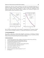
Their numerical results for f"(0) and
0'(0) are shown, for
Pr
= 1, in Figure 1.2 by the solid lines. The exact solution
0'(0) - 0 for rn - _3 is also included in this figure. These quantities are related to
the skin friction ~w at the plate and the heat transfer rate ~w from the plate through
the relations
q-w -kI (~yr )~=0
~UcGr~ x88 f't(O )
l
=
~T*a~88
[-0'(011
(1.35)
We shall further present results for some special values of m.
FREE CONVECTION OVER A VERTICAL FLAT PLATE
13
(~)
4
3.31938 (m - me)-88
0.90819 - 0.28530m + 0.21603m 2
~~i ~'-''" """ t 0.85147m- ~
"=.
~O.90819 - 0.28530m
f u '
mc = -0.9790 m
(b)
e'(o)
2-
rnc = -0.9790
0.11534 (m - me) -~
-0.40103 - 0.31640m + 0.23431m 2
-0.58233 m ~ ]
I i'
"'-" =-:.1L 2 m
,.
~'25.4OlOa - o.a164om
Figure 1.2:
Variation of (a) f" (0), and (b) 0' (0), with m as obtained from numer-
ical integration (solid lines) and asymptotic solutions for Pr = 1. The symbol 9
shows the position of the exact solution 0 ~(0) = 0 for m = 3
5"
14 CONVECTIVE FLOWS
1.3.1 m ,-,~0
An approximate solution of Equations (1.32) - (1.34) near m - 0 can be obtained
by expanding f(~/) and 0(7/) in a power series in m of the form
f(rl)
-
fo(r/)
+ mfl(r/) +
rn2f2(r/) +
0(?7)
O0(f]) -[- ~'t01 (?7) 4- T/%202(7])
-']- 9 9 .
(1.36)
Substituting the expansions (1.36) into Equations (1.32) and (1.33) leads to three
sets of ordinary differential equations which are to be solved subject to the appropri-
ate boundary conditions, which are obtained from the boundary conditions (1.34).
Ingham (1985) has solved these equations numerically and found, for
Pr = 1,
f"(0) - 0.90819 - 0.28530m + 0.21603m 2 +
(1.37)
0'(0)
-
-0.40103
- 0.31640m + 0.23431 m 2 +
for m o 0. This solution is also shown in Figure 1.2.
1.3.2 m >> 1
In this case it is appropriate to make the following transformation
3 1
f-m-ZF(~), 0-0(~), ~-mZ~ (1.38)
This leads to the equations
1 ( 3)FF,
1( 1) F,2
F'"+~ l+ m -~ 1+ +0-0 (1.39)
1( 3)
1 0"+ 1+ FO'-OF'-O
(1.40)
PW ~
where primes now denote differentiation with respect to f and the boundary condi-
tions to be satisfied by these equations are still those given by (1.34). A solution of
Equations (1.39) and (1.40) subject to the boundary conditions (1.34) is sought of
the form
F - Fo (f) + m- 1 F1 (f) + (1.41)
0 O0 (~) -1-/rt-101 (~) -}- 9
where Fo, 0o and F1,01 are given by the equations
Fg' + 88 Fo fg - 89 fg + 0o - 0, ~-~1 e~ + ~ Vo 0; - V~ eo - 0
F0(0) - 0, Fg(0) - 0, 00(0) - 1 (1.42)
F~-+O, 0o-+0 as ~ +cr
F~" + 88 Zo F~' - Vd Z~ + 88 Fd' F~ + 3 Vo Vg - ~ o1~'~ +01 -0
1r
~ ~
+ ~ Fo O l - F; O ~ + ~ Fo O 'o + 88 F, O 'o O o F { -0
F, (0) - 0, F{(0) = 0, 0, (0) - 0 (1.43)
F{ -+0, 01 -'+0 as ~ } oo
FREE CONVECTION OVER A VERTICAL FLAT PLATE 15
It is of some interest to note that Equations (1.42) are the same as those which are
appropriate for a constant plate temperature, the solution of which is well docu-
mented in the papers by Ostrach (1952) and Sparrow and Gregg (1958).
The first set of Equations (1.42) has been solved numerically, for
Pr =
1, by
Ingham (1985), whilst Merkin (19853) has solved both sets of Equations (1.42) and
(1.43) for both
Pr
= 1 and
Pr
# 1. Thus, Merkin (19853) found, for
Pr =
1,
1
f"(O) m ~ (0.8515-0.1579m-1+ )
0'(0)- -m88 (0.5823- 0.0009m-1 + )
(1.44)
for m >> 1.
The large asymptotic values of f"(0) and 0'(0), as given by expressions (1.44),
are compared in Table 1.1 with the values obtained by solving Equations (1.32) -
(1.34) numerically. It is observed that the two values are in good agreement, even
at relatively small values of m.
Table 1.1-
Comparison of f"(O) and
0'(0)
for Pr - 1 as obtained by an exact
solution of Equations (1.32) - (1.3~) and the asymptotic solution (1.4~).
m
1.00
1.25
1.50
1.75
2.00
2.25
2.50
2.75
3.0O
3.25
3.50
3.75
4.00
"[[
Exact
0.7395
0.7155
0.6949
0.6769
0.6611
0.6469
0.6341
0.6225
0.6119
0.6021
0.5931
0.5847
0.576,8
f"(o)
Series (1.44)
0.6936
0.6858
0.6743
0.6619
0.6496
0.6379
0.6269
0.6166
0.6070
0.5980
0.5895
0.5816
0.5742
Exact
0.5951
0.6251
0.6516
0.6754
0.6970
0.7169
0.7354
0.7526
0.7687
0.7839
0.7982
0.8119
0.8249
-o'(o)
Series (1.44)
0.5814
0.6150
0.6438
0.6692
0.6920
0.7132
0.7318
0.7495
0.7660
0.7815
0.7961
0.8100
0.8232
1.3.3 m < 0
From the numerical solution of Equations (1.32) - (1.34) it was observed that as m
decreases below m = 0, the thickness of the boundary-layer decreases, whilst f"(0)
_
3 These
increases and 0t(0) changes sign (from being negative to positive) at m = g.
effects become more pronounced, as rn decreases further and the solution becomes
singular as m approaches a critical value
mc(Pr),
say. This can be clearly seen in
Figure 1.2 and also in Figure 1.3 where the temperature profiles 007 ) are shown for
16 CONVECTIVE FLOWS
__ ,
0 1 2 '7 3
Figure 1.3:
Temperature profiles, O(rl), for Pr- 1 near mc -
-0.9790.
values of m close to
mc -
-0.9790 when
Pr
- 1. To determine the behaviour of
the solution near
mc
it is convenient to introduce the transformation
1 I I
f-e-+G(z), 0-c r z-e-~r/, e-m-m~ (1.45)
where e << 1. Equations (1.32) and (1.33) are thus transformed into the form
1 GG" 1
G,2
G'"+-~(3+mc+e)
-~(l+m~+e) +r
1
r I
Pr
+~(3+mc+e) Gr162
0
(1.46)
(1.47)
with the boundary conditions (1.34) becoming
G(0)- 0, G'(0) =0, r (1.48)
G' +0, r as z-+~
where primes denote differentiation with respect to z.
(1.48) suggest an expansion of the form
The boundary conditions
G - Go(z)-t-eGl(z) }-
. (1.49)
r - r + ~r +
where (Go, r and (G1, r are given by the following equations:
1 (3
+ m~)GoGg G'o 2
Gg' +fiCg - 89 (1+ me) + r = 0
p ~ + 88 (3 + ,~)aor - m~a~r = o
ao(0) = 0, a~(0) = 0, r -
0
a~-+0, r as z +~
(1.50)
FREE CONVECTION OVER A VERTICAL FLAT PLATE 17
V ! __ 1y2!2 __ }GoGg
G~ !' ~- 88 (3 +
mc)(GoG~ -~-
GgG1) - (1 ~-
mc)GoG
1 -~- q~l ~'-~0
p ~ -+- 88 (3 -f- mc)(Gor -I- G1r -
mc
(G~r -~- G~r - G~r - }Gor
GI(0)-0, G~(0)-0, r
G~ +0,
q~l )" 0 aS Z ~ OO
(1.51)
The homogeneous system of Equations (1.50) is an eigenvalue problem for inc.
This system was solved numerically by Ingham (1985) for Pr = 1, whilst Merkin
(1985a) solved it for different values of Pr. Values of mc for various values of
Pr are given in Table 1.2. However, this solution is not unique and will have
G~(O) - Ca, say, for some unknown constant Ca yet to be determined. The value of
Ca is determined from the system (1.51) by writing
1 4 1
Go(5)-C2Go, r 3r GI(g)-CaG1, -2-G 3az (1.52)
where the functions G1 and r satisfy
~tvv
(
)
l ! (
v t 4
1 -~t 2 1 ~ -~l t ~
(J1 -~- 1 (3 + me) GoG1 + G1Go - (1 + mc) GoG 1 + r - C~z ~u 0 - ~t~ot~o)
( -,)
( 1 ,)
Pr
-F 88 (3 +
mc)
(Gor + G1r
-
mc
ator
-t-
GIr
C-~a t-aor
~Gor
GI(O)
O, G 1(0) O, r 1
G 1 + O, (~1 ~0 aS Z ~ O0
(1.53)
and primes now denote differentiation with respect to ~.
Table 1.2" Values of mc and r given by Equation (1.50) for several values of
Pr.
II mo
0.2 -1.1690
0.4 -1.0606
0.6 -1.0204
0.7 -1.0070
0.8 -0.9960
1.0 -0.9790
1.2 -0.9664
1.4 -0.9566
1.6 -0.9487
0.3044
0.4747
0.5930
0.6433
0.6895
0.7729
0.8476
0.9160
0.9794
I gr 11 m~
1
1.8 -0'9422 1.0391
2.0 -0.9368 1.0955
2.5 -0.9263 1.2259
3.0 -0.9188 1.3448
4.0 -0.9086 1.5588
5.0 -0.9019 1.7501
6.0 -0.8971 1.9277
8.0 -0.8907 2.2492
10.0 0.8865 2.5403
,
To solve Equations (1.53) numerically, Merkin (1985a) constructed four separate
solutions, namely two complementary functions (Ga, Ca) and (Gb, Cb) with G~ (0) -
1, r - 0 and G~(0) = 0, r - 1 and two particular integrals (Go, r which
is a solution of the system (1.53) with the right-hand sides set to zero but with
G~(0) - 0, r - 1 and r = 0 and (Cd, Cd), which is a solution of the full
18 CONVECTIVE FLOWS
4
Equations (1.53) with C2 replaced by 1 and G~(0) - Cd(0) r 0.
complete solution is then given by
The
4
G1 - o~aGa + o~bGb + Gc + Ca 3 Gd
4
~)1 Ot a ~) a ~- Ol b ~) b -~- ~P c -Jr 6a 3 (~ d
(1.54)
with aa and
O~ b
being additional constants.
After some manipulations, Merkin (1985a) found that
Ca
is given by
4 AbBc- AcBb
C~ = AdBb- AbBd
(1.55)
where
Ai
and Bi (i - a, b, c, d) are constants, which are obtained from the system
(1.53) if we note that r + Ai and
G~ ~ -Ai-z + Bi
as ~ -+ co.
Finally, we have
3
f"(O) - Ca (m- me) -~ +
0'(0) - 0.7729
Ca (m - me)
5
4 ~- . . .
(1.56)
as
m -+ mc(Pr).
For
Pr
- 1 it was found by Merkin (1985a) that
Ca -
0.31943
and
mc -
-0.9790, so that the expressions (1.56) become
3
f"(O) - 0.31943(rn- me) 4 +
5
0'(0) 0.24688
(m mc) -~ +
(1.57)
as
m + mc-
-0.9790. However, Ingham (1985) found, for
Pr- 1,
f"(0) = 0.31938 (m - m~)
0'(0)
- 0.11534 (m - m~)
3
4 ~
(1.58)
4 ~
as rn -~
mc -
-0.9790 and this solution is also shown in Figure 1.2. We note
that there is a very good agreement between the asymptotic solution (1.58) and the
numerical solution of Equations
(1.32)
- (1.34).
1.4
Similarity solutions for an impermeable fiat plate
with a variable surface heat flux
In this case, from Equation (1.30), we have
N(x)
= 0 and assume that the heat flux
qw(X)
at the plate is of the form
qw(X) = x
TM
(1.59)
FREE CONVECTION OVER A VERTICAL FLAT PLATE 19
which gives
Q(x) - m.
The non-dimensional variables (1.26) now take the form
x(4+m )
1 l(m_l )
r X5 f(r]), T xs(l+4m)o(r]), ?7 yxg
(1.60)
so that Equations (1.27) and (1.28) become
1 f,, 1 (3 + 2m)f '2 + 0 - 0
f'" + ~(4 +
m)f - -~
1 1
1 0"+ (4+m)fO'- (l+4m)f'O-O
P 7 g g
which have to be solved subject to the boundary conditions
(1.61)
(1.62)
f(0)-0, f'(0) 0, 0'(0) 1 (163)
f' + O, 0 +0
as r/-~c~
It should be noted that the case m - 0 (uniform surface heat flux) was considered
by Sparrow and Gregg (1956).
Equations (1.61) - (1.63) can be integrated in a similar way to those given by
Equations (1.32) - (1.34) for the prescribed surface temperature case. Thus, a
solution is first obtained for m >> 1 by using the transformation
4 1 1
f-m
5f(~), 0-m 50(~), ~-m~r/ (1.64)
The transformed equations for f (~) and 0 (~) were solved numerically by Merkin
(1985a), again for
Pr
- 1. Thus, the asymptotic expressions for the reduced skin
friction f"(0) and reduced wall temperature 0(0) are given by
2
f"(0)- m-~ (1.2878-
0.4257m-1 ~ )
0(0)- m-~ (1.6116- 0.0780m-1 + )
as rn + cx). Values of f"(0) and 0(0), as given by expressions (1.65), as a function of
m are presented in Table 1.3, together with their values obtained from a numerical
integration of Equations (1.61) - (1.63). It is seen again that the two sets of values
are in good agreement, even for moderate values of m.
The situation for m < 0 is slightly different to the prescribed temperature case.
Again, as m decreases from m - 0, the thickness of the boundary-layer decreases
and both f"(0) and 0(0) increase, and approach a singularity as m tends to minus
unity, as can be seen in Figure 1.4. However, we can show that Equations (1.61) and
(1.62) cannot have a solution when m = -1. Indeed, with m - -1, Equation (1.62)
can be integrated once to give
10 ,
+
5f0-
constant (1.66)
Pr
where this constant cannot be chosen to be compatible with the boundary conditions
(1.63) on both 77 - 0 and as r/ -~ co. In fact, Equations (1.61) and (1.62) cannot