Heat Transfer: Basics and Practice ppt
Bạn đang xem bản rút gọn của tài liệu. Xem và tải ngay bản đầy đủ của tài liệu tại đây (4.24 MB, 291 trang )
Heat Transfer
•Peter von Böckh Thomas Wet elz
Heat Transfer
Basics and Practice
Prof. Dr. Peter von Böckh Prof. Dr Ing. Thomas Wetzel
Hedwig-Kettler-Str. 7 Karlsruhe Institute of Technology
76137 Karlsruhe KIT
Germany Kaiserstr. 12
76128 Karlsruhe
Germany
ISBN 978-3-642-19182-4 e-ISBN 978-3-642-19183-1
DOI 10.1007/978-3-642-19183-1
Springer Heidelberg Dordrecht London New York
Library of Congress Control Number: 2011940209
¤ Springer-Verlag Berlin Heidelberg 2012
This work is subject to copyright. All rights are reserved, whether the whole or part of the material is
concerned, specifically the rights of translation, reprinting, reuse of illustrations, recitation,
broadcasting, reproduction on microfilm or in any other way, and storage in data banks. Duplication
of this publication or parts thereof is permitted only under the provisions of the German Copyright
Law of September 9, 1965, in its current version, and permission for use must always be obtained
from Springer. Violations are liable to prosecution under the German Copyright Law.
The use of general descriptive names, registered names, trademarks, etc. in this publication does not
imply, even in the absence of a specific statement, that such names are exempt from the relevant
protective laws and regulations and therefore free for general use.
Printed on acid-free paper
Springer is part of Springer Science+Business Media (www.springer.com)
Preface
This book is the English version of the fourth edition of the German book
“Wärmeübertragung”. I originally wrote the book based on my lecture notes. In my
work with Asea Brown Boveri until 1991 I was closely involved with the design and
development of heat exchangers for steam power plants. There the latest research
results were required in the area of heat transfer, to develop new and more exact
calculation procedures. In this business an accuracy of 0.5 % was required in order
to be competitive.
However, although our young engineers were full theoretical knowledge about
boundary layers, analogy theorems and a large number of calculation procedures,
but could not design a very simple heat exchanger.
Later in my professorship at the University of Applied Sciences in Basel
(Switzerland), I noticed that the most books for students on heat transfer were not
up to date. Especially the American books with excellent didactic features, did not
represent the state of the art in many fields. My lecture notes – and so this book –
were then developed with the aim providing the students with state of the art
correlations and enable them to really design and analyzing heat exchangers.
The VDI Heat Atlas presents the state of the art in heat transfer, but it is an
expert’s reference, too large and not instructive enough for students. It is used
therefore frequently as a source in this book, but here we focus more on a didactic
way of presenting the essentials of heat transfer along with many examples.
The first edition of this book was published in 2003. At the University of
Applied Science in Basel after 34 lectures of 45 minutes the students could
independently recalculate and design fairly complex heat exchangers, e.g. the
cooling of a rocket combustion chambers, evaporators and condensers for heat
pumps.
After my retirement Professor Thomas Wetzel, teaching Heat and Mass Transfer
at Karlsruhe Institute of Technology (KIT), joined me as co-author. He is professor
at the Institute of Thermal Process Engineering, the institute where large parts of
the correlations in VDI Heat Atlas were developed. His professional background
(heat transfer in molten semi-conductor materials, automotive compact heat
exchangers and air conditioning, chemical process engineering) is complementary
to my experience.
This book requires a basic knowledge of thermodynamics and fluid mechanics,
e.g. first law of thermodynamics, hydraulic friction factors.
v
vi
The examples in the book solved with Mathcad 14, can be down loaded from
www.waermeuebertragung-online.de or www.springer.com/de/978-3-642-15958-
9. The downloaded modules can be used for heat exchanger design. Also polinoms
for material properties as described in Chapter 9 are programmed in Mathcad 14
and can so be implemented in other Mathcad 14 programs for the call of material
properties of water, air and R134a.
We have to thank Prof. von Böckh’s wife Brigitte for her help in completing
this book. She spent a great deal of time on reviewing the book. She checked the
correct size and style of letters, use of symbols, indices and composition. The
appearance of the layout and legibility of the book is mainly her work.
Peter von Böckh with Thomas Wetzel, Karlsruhe, August 2011
Preface
Contents
List of ymbols xi
1 Introduction and definitions 1
1.1 Modes of heat transfer 3
1.2 Definitions 4
1.2.1 Heat (transfer) rate and heat flux 4
1.2.2 Heat transfer coefficients and overall heat transfer coefficients 4
1.2.3 Rate equations 6
1.2.4 Energy balance equations 6
1.2.5 Log mean temperature difference 7
1.2.6 Thermal conductivity 9
1.3 Methodology of solving problems 9
2 Thermal conduction in static materials 17
2.1 Steady-state thermal conduction 17
2.1.1 Thermal conduction in a plane wall 18
2.1.2 Heat transfer through multiple plane walls 22
2.1.3 Thermal conduction in a hollow cylinder 25
2.1.4 Hollow cylinder with multiple layers 29
2.1.5 Thermal conduction in a hollow sphere 32
2.1.6 Thermal conduction with heat flux to extended surfaces 35
2.1.6.1 Temperature distribution in the fin 36
2.1.6.2 Temperature at the fin tip 38
2.1.6.3 Heat rate at the fin foot 38
2.1.6.4 Fin efficiency 39
2.1.6.5 Applicability for other geometries 40
2.2 Transient thermal conduction 44
2.2.1 One-dimensional transient thermal conduction 44
2.2.1.1 Determination of the temporal change of temperature 44
2.2.1.2 Determination of transferred heat 47
2.2.1.3 Special solutions for short periods of time 58
2.2.2 Coupled systems 60
2.2.3 Special cases at Bi = 0 and Bi =
∞
62
vii
S
viii Contents
2.2.4 Temperature changes at small Biot numbers 62
2.2.4.1 A small body immersed in a fluid with large mass 63
2.2.4.2 A body is immersed into a fluid of similar mass 65
2.2.4.3 Heat transfer to a static fluid by a flowing heat carrier 68
2.2.5 Numerical solution of transient thermal conduction equations 70
2.2.5.1 Discretization 70
2.2.5.2 Numerical solution 73
2.2.5.3 Selection of the grid spacing and of the time interval 74
3 Forced convection 77
3.1 Dimensionless parameters 78
3.1.1 Continuity equation 79
3.1.2 Equation of motion 80
3.1.3 Equation of energy 81
3.2 Determination of heat transfer coefficients 83
3.2.1 Flow in a circular tube 83
3.2.1.1 Turbulent flow in circular tubes 83
3.2.1.2 Laminar flow in circular tubes at constant wall temperature 85
3.2.1.3 Equations for the transition from laminar to turbulent 86
3.2.1.3 Flow in tubes and channels of non-circular cross-sections 94
3.2.2 Flat plate in parallel flow 98
3.2.3 Single bodies in perpendicular cross-flow 99
3.2.4 Perpendicular cross-flow in tube bundles 103
3.2.5 Tube bundle with baffle plates 109
3.3 Finned tubes 110
3.3.1 Annular fins 112
4 Free convection 119
4.1 Free convection at plain vertical walls 120
4.1.1 Inclined plane surfaces 126
4.2 Horizontal plane surfaces 128
4.3 Free convection on contoured surface areas 128
4.3.1 Horizontal cylinder 129
4.3.2 Sphere 130
4.4 Interaction of free and forced convection 130
5 Condensation of pure vapors 131
5.1 Film condensation of pure, static vapor 131
5.1.1 Laminar film condensation 131
5.1.1.1 Condensation of saturated vapor on a vertical wall 131
5.1.1.2 Influence of the changing wall temperature 135
5.1.1.3 Condensation of wet and superheated vapor 136
5.1.1.4 Condensation on inclined walls 137
5.1.1.5 Condensation on horizontal tubes 137
ixContents
5.1.2 Turbulent film condensation on vertical surfaces 137
5.2 Dimensionless similarity numbers 137
5.2.1 Local heat transfer coefficients 138
5.2.2 Mean heat transfer coefficients 139
5.2.3 Condensation on horizontal tubes 139
5.2.4 Procedure for the determination of heat transfer coefficients 140
5.2.5 Pressure drop in tube bundles 147
5.3 Condensation of pure vapor in tube flow 151
5.3.1 Condensation in vertical tubes 152
5.3.1.1 Parallel-flow (vapor flow downward) 153
5.2.1.2 Counterflow (vapor flow upward) 154
5.3.2 Condensation in horizontal tubes 158
6 Boiling heat transfer 171
6.1 Pool boiling 171
6.1.1 Sub-cooled convection boiling 173
6.1.2 Nucleate boiling 173
6.2 Boiling at forced convection 182
6.2.1 Sub-cooled boiling 182
6.2.2 Convection boiling 183
7 Thermal radiation 189
7.1 Basic law of thermal radiation 190
7.2 Determination of the heat flux of radiation 191
7.2.1 Intensity and directional distribution of the radiation 192
7.2.2 Emissivities of technical surfaces 193
7.2.3 Heat transfer between two surfaces 194
7.2.3.1 Parallel gray plates with identical surface area size 196
7.2.3.2 Surrounded bodies 197
7.3 Thermal radiation of gases 206
7.3.1 Emissivities of flue gases 207
7.3.1.1 Emissivity of water vapor 207
7.3.1.2 Emissivity of carbon dioxide 208
7.3.2 Heat transfer between gas and wall 208
8 Heat exchangers 215
8.1 Definitions and basic equations 215
8.2 Calculation concepts 218
8.2.1 Cell method 218
8.2.2 Analysis with the log mean temperature method 223
8.3 Fouling resistance 236
8.4 Tube vibrations 240
8.4.1 Critical tube oscillations 240
8.4.2 Acoustic resonance 242
x Contents
Appendix 245
A1: Important physical constants 245
A2: Thermal properties of sub-cooled water at 1 bar pressure 246
A3: Thermal properties of saturated water and steam 248
A4: Thermal properties of water and steam 250
A5: Thermal properties of saturated Freon 134a 252
A6: Thermal properties of air at 1 bar pressure 254
A7: Thermal properties of solid matter 255
A8: Thermal properties of thermal oils 256
A9: Thermal properties of fuels at 1.013 bar 257
A10: Emissivity of surfaces 258
A11: Formulary 261
Index 275
Bibliography 271
List of Symbols
a thermal difusivity m
2
/s
a = s
1
/d dimensionless tube distance perpendicular to flow -
A flow cross-section, heat transfer area, surface area m
2
Bi Biot number -
B, b width m
b = s
2
/d dimensionless tube distance parallel to flow -
C
12
radiation heat exchange coefficient W/(m
2
K
4
)
C
s
Stefan-Boltzmann-constant of black bodies 5.67 W/(m
2
K
4
)
c flow velocity m/s
c
0
cross-flow inlet velocity m/s
c
p
specific heat at constant pressure J/(kg K)
D, d diameter m
d
A
bubble tear-off diameter m
d
h
hydraulic diameter m
F force N
F
s
gravity force N
F
τ
sheer stress force N
Fo Fourier number -
f
1
, f
2
correction functions of heat transfer coefficients -
f
A
correction function for tube arrangement in a tube bundle -
f
j
, f
n
correction function for first row effect in tube bundles -
g gravitational acceleration 9,806 m/s
2
Gr Grashof number -
H height of a tube bundle m
H = m
.
h enthalpy J
h Planck-constant 6,6260755
.
10
-34
J
.
s
h specific enthalpy J/kg, kJ/kg
h fin height m
i number of tubes per tube row -
i
λ
,s
spectral specific intensity of black radiation W/m
3
k overall heat transfer coefficient W/(m
2
K)
k Boltzmann-constant 1.380641
.
10
-23
J/K
L' = A/U
proj
flow length m
3
2
/
ν
gL' =
characteristic length of condensation m
l length m
m mass kg
xi
xii
m characteristic fin parameter m
-1
m
mass flow rate kg/s
NTU number of transfer units -
Nu Nußelt number -
n number of tube rows, number of fins -
p pressure Pa, bar
P dimensionless temperature -
Pr Prandtl number -
Q heat J
Q
heat rate W
q
heat flux W/m
2
R individual gas constant J/(kg K)
R
m
universal gas constant J/(mol K)
R
a
mean roughness index m
R
v
fouling resistance (m
2
K)/W
r radius m
r latent heat of evaporation J/kg
R
1
ratio of heat capacity rate of fluid 1 to fluid 2 -
Ra Rayleigh number -
Re Reynolds number -
s
1
tube distance perpendicular to flow m
s
2
tube distance parallel to flow m
s wall thickness m
s
Ri
fin thickness
T absolute temperature K
T
i
dimensionless temperature -
t time s
t
Ri
fin distance m
V volume m
3
p
cmW ⋅=
heat capacity rate W/K
X characteristic parameter for fin efficiency -
x steam quality -
x, y, z spacial coordinates m
α
x
local heat transfer coefficients W/(m
2
K)
α
mean heat transfer coefficients W/(m
2
K)
α
absorptivity -
β
thermal expansivity 1/T
β
0
bubble contact angle °
δ
thickness of condensate film m
δ
ϑ
thickness of thermal boundary layer m
ε
emissivity -
Δϑ
temperature difference K
Δϑ
gr
, Δϑ
kl
larger and smaller temperature difference at inlet and outlet K
List of ymbolsS
xiii
Δϑ
m
log mean temperature difference K
ϑ
Celsius temperature °C
ϑ
',
ϑ
'' inlet resp. outlet temperature °C
Θ
dimensionless temperature -
η
Ri
fin efficiency -
η
dynamc viscosity kg/(m s)
ν
kinematc viscosity m
2
/s
λ
thermal conduction W/(m K)
λ
wave length m
ρ
density kg/m
3
σ
surface tension N/m
σ
Stefan-Boltzmann-constant 5.6696
.
10
-8
W/(m
2
K
4
)
τ
sheer stress N/m
2
Ψ
hollow volume ratio, porosity -
ξ
resistance factor -
Indexes
1, 2, state, fluid
12, 23, change of state from 1 to 2
A state at start of transient thermal conduction at time t = 0
A bouyancy
a outlet, outside
e inlet
f fluid
f 1, f 2 fluid 1, fluid 2
g gas
i inside
l liquid
lam laminar
m mean value
m middle
n normal component of a vector
O surface
r radial component of a vector
Ri fin
s black body
turb turbulent
W wall
x local value at location x, steam quality
x, y, zx-, y- und z-components of a vector
List of ymbolsS
1 Introduction and definitions
Heat transfer is a fundamental part of thermal engineering. It is the science of the rules
governing the transfer of heat between systems of different temperatures. In thermo-
dynamics, the heat transferred from one system to its surroundings is assumed as a
given process parameter. This assumption does not give any information on how the
heat is transferred and which rules determine the quantity of the transferred heat.
Heat transfer describes the dependencies of the heat transfer rate from a corre-
sponding temperature difference and other physical conditions.
The thermodynamics terms “control volume” and “system” are also common in heat
transfer. A system can be a material, a body or a combination of several materials or
bodies, which transfer to or receive heat from another system.
The first two questions are:
• What is heat transfer?
• Where is heat transfer applied?
Heat transfer is the transport of thermal energy, due to a spacial temperature
difference.
If a spacial temperature difference is present within a system or between sys-
tems in thermal contact to each other, heat transfer occurs.
The application of the science of heat transfer can be easily demonstrated with the
example of a radiator design.
Room temperature
Heat rate
Radiator surface area
Inlet temperature
ϑ
Mass flow rate
m
.
in
Heating water
ϑ
R
A
Q
.
Figure 1.1: Radiator design
P. von Böckh and T. Wetzel, Heat Transfer: Basics and Practice,
1
DOI 10.1007/978-3-642-19183-1_1, © Springer-Verlag Berlin Heidelberg 2012
2 1 Introduction and definitions
To obtain a certain room temperature, radiators, in which warm water flows, are
installed to provide this temperature. For the acquisition of the radiators, the
architect defines the required heat flow rate, room temperature, heating water mass
flow rate and temperature. Based on these data, the radiator suppliers make their
offers. Is the designed radiator surface too small, temperature will be too low, the
owner of the room will not be satisfied and the radiator must be replaced. Is the
radiator surface too large, the room temperature will be too high. With throttling the
heating water flow rate the required room temperature can be established. However,
the radiator needs more material and will be too expensive, therefore it will not be
ordered. The supplier with the correct radiator size will succeed. With experiments the
correct radiator size could be obtained, but this would require a lot of time and costs.
Therefore, calculation procedures are required, which allow the design of a radiator
with an optimum size. For this example, the task of heat transfer analysis is to obtain
the correct radiator size at minimum costs for the given parameters .
In practical design of apparatus or complete plants, in which heat is transferred,
besides other technical sciences (thermodynamics, fluid mechanics, material science,
mechanical design, etc.) the science of heat transfer is required. The goal is always to
optimize and improve the products. The main goals are to:
• increase efficiency
• optimize the use of resources
• reach a minimum of environmental burden
• optimize product costs.
To reach these goals, an exact prediction of heat transfer processes is required.
To design a heat exchanger or a complete plant, in which heat is transferred,
exact knowledge of the heat transfer processes is mandatory to ensure the
greatest efficiency and the lowest total costs.
Table 1.1 gives an overview of heat transfer applications.
Table 1.1: Area of heat transfer applications
Heating, ventilating and air conditioning systems
Thermal power plants
Refrigerators and heat pumps
Gas separation and liquefaction
Cooling of machines
Processes requiring cooling or heating
Heating up or cooling down of production parts
Rectification and distillation plants
Heat and cryogenic isolation
Solar-thermic systems
Combustion plants
1 Introduction and definitions 3
1.1 Modes of heat transfer
Contrary to assured knowledge, most publications describe three modes of heat
transfer: thermal conduction, convection and thermal radiation.
Nußelt, however, postulated in 1915, that only two modes of heat transfer exist [1.2]
[1.3]. The publication of Nußelt states:
“In the literature it is often stated, heat emission of a body has three causes: radiation,
thermal conduction and convection.
The separation of heat emission in thermal conduction and convection suggests that
there would be two independent processes. Therefore, the conclusion would be: heat
can be transferred by convection without the participation of thermal conduction. But
this is not correct.”
Heat transfer modes are thermal conduction and thermal radiation.
Figure 1.2 demonstrates the two modes of heat transfer.
ϑ
to a moving fluid (convection)
Thermal conduction from a surface
ϑ
>
.
.
Thermal conduction in a solid
material or static fluid
Q
ϑ
2
ϑ
1
>
ϑ
1
ϑ
2
ϑ
.
.
Q
1
Moving fluid
radiation between two surfaces
Heat transfer by thermal
1
>
ϑ
1
ϑ
2
2
ϑ
2
Q
1
.
.
ϑ
.
.
2
Q
1
ϑ
2
Figure 1.2: Modes of heat transfer
1. Thermal conduction develops in materials when a spacial temperature gradi-
ent is present. With regard to calculation procedures there is a differentiation
between static materials (solids and static fluids) and moving fluids. Heat
transfer in static materials depends only on the spacial temperature gradient
and material properties.
Heat transfer between a solid wall and a moving fluid occurs by thermal con-
duction between the wall and the fluid and within the fluid. Furthermore, the
transfer of enthalpy happens, which mixes areas of different temperatures.
The heat transfer is determined by the thermal conductivity and the thickness
of the boundary layer of the fluid, the latter is dependent on the flow and
material parameters. In the boundary layer the heat is transferred by conduc-
tion.
Because of the different calculation methods, the heat transfer between a
solid wall and a fluid is called convective heat transfer or more concisely
convection. A further differentiation is made between free convection and
forced convection.
4 1 Introduction and definitions
In free convection the fluid flow is generated by gravity due to the density
difference caused by the spacial temperature gradient. At forced convection
the flow is established by an external pressure difference.
2. Thermal radiation can occur without any intervening medium. All surfaces
and gases consisting of more than two atoms per molecule of finite tempera-
ture, emit energy in the form of electromagnetic waves. Thermal radiation is a
result of the exchange of electromagnetic waves between two surfaces of
different temperature.
In the examples shown in Figure 1.3 the temperature
ϑ
1
is larger than
ϑ
2
, therefore,
the heat flux is in the direction of the temperature
ϑ
2
. In radiation both surfaces emit
and absorb a heat flux, where the emission of the surface with the higher temperature
ϑ
1
has a higher intensity.
Heat transfer may occur through combined thermal conduction and radiation. In
many cases, one of the heat transfer modes is negligible. The heat transfer modes of
the radiator, discussed at the beginning of this chapter are: forced convection inside
from the water to the inner wall, thermal conduction in the solid wall and a combina-
tion of free convection and radiation from the outer wall to the room.
The transfer mechanism of the different heat transfer modes are governed by differ-
ent physical rules and therefore, their calculation methods will be discussed in sepa-
rate chapters.
1.2 Definitions
The parameters required to describe heat transfer will be discussed in the following
chapters.
In this book the symbol
ϑ
is used for the temperature in Celsius and T for the
absolute temperature.
1.2.1 Heat (transfer) rate and heat flux
The heat rate, also called heat transfer rate
Q
is the amount of heat transferred
per unit time. It has the unit Watt W.
A further important parameter is the heat flux density
AQq /
=
, which defines the
heat rate per unit area. Its unit is Watt per square meter W/m
2
.
1.2.2 Heat transfer coefficients and overall heat transfer coefficients
The description of the parameters, required for the definition of the heat flux density
will be discussed in the example of a heat exchanger as shown in Figure 1.3. The heat
exchanger consist of a tube that is installed in the center of a larger diameter tube.
1 Introduction and definitions 5
A fluid with the temperature
ϑ
1
' enters the inner tube and will be heated up to the
temperature
ϑ
1
''. In the annulus a warmer fluid will be cooled down from the
temperature
ϑ
2
' to the temperature
ϑ
2
''. Figure 1.3 shows the temperature profiles in
the fluids and in the wall of the heat exchanger.
The governing parameters for the heat rate transferred between the two fluids will be
discussed now. The quantity of the transferred heat rate
Q
can be defined by the
heat transfer coefficient
α
, the heat transfer surface area A and the temperature
difference
Δϑ
.
The heat transfer coefficient defines the heat rate
Q
transferred per unit
transfer area A and per unit temperature difference
Δϑ
.
The unit of the heat transfer coefficient is W/(m
2
K).
system boundary
x
.
m
ϑ
'
2
ϑ
'
1
ϑ
ϑ
'
2
2
ϑ
'
1
m
.
1
Y
dx
1
ϑ
''
ϑ
''
2
x
1
Y
ϑ
ϑ
W
1
ϑ
''
1
ϑ
W
2
ϑ
2
ϑ
''
2
.
Q
Figure 1.3: Temperature profile in the heat exchanger
With this definition, the finite heat rate through a finite surface element is:
22222
)( dAQ
W
⋅−⋅=
ϑϑαδ
(1.1)
11111
)( dAQ
W
⋅−⋅=
ϑϑαδ
(1.2)
WWWWW
dAQ ⋅−⋅= )(
12
ϑϑαδ
(1.3)
The symbol
Q
δ
shows that the heat rate has an inexact differential, because the
value of its integral depends on the heat transfer processes and path.
The integral of
Q
δ
is
12
Q
and not
21
QQ−
.
6 1 Introduction and definitions
Here the temperature differences were selected such that the heat rate has positive
values. For a heat exchanger with a complete thermal insulation to the environment,
the heat rate coming from fluid 2 must have the same value as the one transferred to
fluid 1 and also have the same value as the heat rate through the pipe wall.
QQQQ
W
δδδδ
===
21
(1.4)
In most cases, the wall temperatures are unknown and the engineer is interested in
knowing the total heat rate transferred from fluid 2 to fluid 1. For its determination the
overall heat transfer coefficient k is required. It has the same unit as the heat transfer
coefficient.
dAkQ ⋅−⋅= )(
12
ϑϑδ
(1.5)
Using equations (1.1) to (1.5) the relationships between the heat transfer and over-
all heat transfer coefficients can be determined. It has to be taken into account that
the surface area in- and outside of the tube has a different magnitude. The determina-
tion of the overall heat transfer coefficient will be shown in the following chapters.
In this chapter the heat transfer coefficients are assumed to be known values.
In the following chapters the task will be to determine the heat transfer coeffi-
cient as a function of material properties, temperatures and flow conditions of
the involved fluids.
1.2.3 Rate equations
Equations (1.1) to (1.3) and (1.5) define the heat rate as a function of heat transfer
coefficient, surface area and temperature difference. They are called rate equations.
The rate equations define the heat rate, transferred through a surface area at
a known heat transfer coefficient and a temperature difference.
1.2.4 Energy balance equations
In heat transfer processes the first law of thermodynamics is valid without any re-
strictions. In most practical cases of heat transfer analysis, the mechanical work,
friction, kinetic and potential energy are small compared to the heat rate. Therefore,
for problems dealt with in this book, they are neglected. The energy balance
equation of thermodynamics then simplifies to [1.1]:
CV
CV e e a a
ea
dE
Qmhmh
dt
=+ ⋅− ⋅
¦¦
(1.6)
The temporal change of energy in the control volume is equal to the total heat rate
to the control volume and the enthalpy flows to and from the control volume. In most
1 Introduction and definitions 7
cases of heat transfer problems only one mass flow enters and leaves a control
volume. The change of the enthalpy and energy in the control volume can be given as
a function of the temperature. The heat rate is either transferred over the system
boundary or originates from an internal source within the system boundary (e.g.
electric heater, friction, chemical reaction). Equation (1.7) is presented here as it is
mostly used for heat transfer problems:
12 2 1
()
CV p in
d
Vc QQmhh
dt
ϑ
ρ
⋅⋅ = + + ⋅ −
(1.7)
In Equation (1.7)
12
Q
is the heat rate transferred over the system boundary and
in
Q
the heat rate originating from an internal source. For stationary processes the left
side of Equation (1.7) has the value of zero:
12 1 2 1 2
() ( )
in p
QQ mhh mc
ϑϑ
+=⋅−=⋅⋅−
(1.8)
The Equations (1.7) and (1.8) are called energy balance equations.
1.2.5 Log mean temperature difference
With known heat transfer coefficients, the heat rate at every location of the heat
exchanger, shown in Figure 1.3, can be determined. In engineering, however, not the
local but the total transferred heat is of interest. To determine the overall heat transfer
rate, the local heat flux density must be integrated over the total heat transfer area.
The total transferred heat rate is:
dAkQ
A
⋅−⋅=
³
)(
12
0
ϑϑ
(1.9)
The variation of the temperature in the surface area element dA can be calculated
using the energy balance equation (1.8).
11 11 1p
Qmdh mc d
δϑ
=⋅ =⋅⋅
(1.10)
22 22 2p
Qmdh mcd
δϑ
=− ⋅ =− ⋅ ⋅
(1.11)
The temperature difference
ϑ
2
–
ϑ
1
will be replaced by
Δϑ
. The change of the
temperature difference can be calculated from the change of the fluid temperatures.
¸
¸
¹
·
¨
¨
©
§
⋅
+
⋅
⋅−=−=
2211
12
11
pp
cmcm
Qddd
δϑϑϑΔ
(1.12)
Equation (1.12) set in Equation (1.5) results in:
8 1 Introduction and definitions
dA
cmcm
k
d
pp
⋅
¸
¸
¹
·
¨
¨
©
§
⋅
+
⋅
⋅−=
2211
11
ϑΔ
ϑΔ
(1.13)
Assuming that the overall heat transfer coefficient, the surface area and the spe-
cific heat capacities are constant, Equation (1.13) can be integrated. This assumption
will never be fulfilled exactly. However, in practice the use of mean values has proven
to be an excellent approach. The integration gives us:
¸
¸
¹
·
¨
¨
©
§
⋅
+
⋅
⋅⋅=
¸
¸
¹
·
¨
¨
©
§
′′
−
′′
′
−
′
221112
12
11
ln
pp
cmcm
Ak
ϑϑ
ϑϑ
(1.14)
With the assumptions above, Equations (1.10) and (1.11) can also be integrated.
)(
1111
ϑϑ
′
−
′′
⋅⋅=
p
cmQ
(1.15)
)(
2222
ϑϑ
′′
−
′
⋅⋅=
p
cmQ
(1.16)
In Equation (1.14) the mass flow rates and specific heat capacities can be replaced
by the heat rate and fluid temperatures. This operation delivers:
2121
21
21
ln
m
QkA kA
ϑϑϑϑ
Δϑ
ϑϑ
ϑϑ
′′′′′′
−−+
=⋅⋅ =⋅⋅
′′
−
′′ ′′
−
(1.17)
The temperature difference
m
Δϑ
is the temperature difference relevant for the
estimation of the heat rate. It is called the log mean temperature difference
and is the integrated mean temperature difference of a heat exchanger.
The log mean temperature difference is valid for the special case of the heat
exchanger shown in Figure 1.3. For heat exchanger with parallel-flow, counterflow
and if the temperature of one of the fluids remains constant (condensation and boil-
ing) a generally valid log mean temperature difference can be given. For its formula-
tion the temperature differences at the inlet and outlet of the heat exchangers are
required. The greater temperature difference is
Δϑ
gr
, the smaller one is
Δϑ
sm
.
if 0
ln( / )
gr sm
mgrsm
gr sm
Δϑ Δϑ
Δϑ Δϑ Δϑ
Δϑ Δϑ
−
=−≠
(1.18)
If the temperature differences at inlet and outlet are approximately identical, Equa-
tion (1.18) results in an indefinite value. For this case the log mean temperature diffe-
rence is the average value of the inlet and outlet temperature differences.
()/2if 0
mgrkl grkl
Δϑ Δϑ Δϑ Δϑ Δϑ
=+ −=
(1.19)
1 Introduction and definitions 9
The log mean temperature of a heat exchanger in which the flow of the fluids is
perpendicular (cross-flow) or has changing directions will be discussed in Chapter 8.
1.2.6 Thermal conductivity
Thermal conductivity
λ
is a material property, which defines the magnitude of the
heat rate that can be transferred per unit length in the direction of the flux and per unit
temperature difference. Its unit is W/(m K). The thermal conductivity of a material is
temperature and pressure dependent.
Good electric conductors are usually also good thermal conductors, however, ex-
ceptions exist. Metals have a rather high thermal conductivity, liquids a smaller one
and gases are “bad” heat conductors. In Figure 1.4 thermal conductivity of several
materials is plotted versus temperature.
The thermal conductivity of most materials does not vary much at a medium tem-
perature change. Therefore, they are suitable for calculation with constant mean
values.
1.3 Methodology of solving problems
This chapter originates from [1.5], with small changes. For solving problems of heat
transfer usually, directly or indirectly, the following basic laws and principles are
required:
• law of Fourier
• laws of heat transfer
• conservation of mass principle
• conservation of energy principle (first law of thermodynamics)
• second law of thermodynamics
• Newton’s second law of motion
• momentum equation
• similarity principles
• friction principles
Besides profound knowledge of the basic laws, the engineer has to know the
methodology, i.e. how to apply the above mentioned basic laws and principles to
concrete problems. It is of great importance to learn a systematic analysis of prob-
lems. This consist mainly of six steps as listed below. They are proven in practice
and can, therefore, highly be recommended.
10 1 Introduction and definitions
Fig. 1.4: Thermal conductivity of materials versus temperature [1.5]
Ferritic steels
A
u
s
t
e
n
i
t
i
c
s
t
e
e
l
s
Q
u
a
r
t
z
g
la
s
s
Temperature in °C
Thermal conductivity in W / (m K)
-100
0,01
0.02
0.04
0.06
0.08
0.1
-40-60-80
0
-20 20
Criogenic insulation,
cork, foam
0.6
0.2
0.4
1
2
0.8
O
r
g
a
n
i
c
f
l
u
i
d
s
6
4
8
10
20
40
Ic
e
100
200
60
80
400
400
800
1 000
H
e
a
t
i
n
s
u
l
a
t
i
o
n
(
m
i
n
e
r
a
l
f
i
b
r
e
)
600
W
a
t
e
r
v
a
p
o
r
a
t
1
b
a
r
200
100
40 8060 400
A
i
r
800
1 000
H
e
l
i
u
m
H
y
d
r
o
g
e
n
Stones
Water
A
l
u
m
i
n
u
m
Silver
G
o
l
d
Copper