process control systems application design and adjustment
Bạn đang xem bản rút gọn của tài liệu. Xem và tải ngay bản đầy đủ của tài liệu tại đây (4.26 MB, 376 trang )
Application
F. G.
SHINSKEY
Systems Design Engineer, The Foxboro Company
“\
I
M C GRAW-HILL
BOOK COMPANY
a
New York
San Francisco
Toronto
London Sydney
•
"
u.
P
nl
�
·
.•
. . .
viii
I
Preface
are not communicated to the people who must apply them. Control
problems arise in the plant and must be solved in the plant. Until plant
engineers and control designers are able to communicate with each
other, their mutual problems await solution. I do not mean to imply
that abstract mathematics is not capable of solving control problems, but
it is striking how often the same solution can be reached by using good
common sense. High-order equations and high-speed computers can
be manipulated to the point where common sense is dulled.
Some months ago I was asked to give a course on process control to
a large group of engineers from various departments of The Foxboro
Company. Sales, Product Design, Research, Quality Control, and
Project Engineering were all to be represented. If the subject were
presented through the traditional medium of operational calculus, the
effort would be wasted, because too few of the students would have this
prerequisite. Rather than attempt to teach operational calculus, I
chose to do without it altogether.
It then became necessary to approach
control problems solely in the time domain. Once the transition was
begun, I was surprised at the fresh point of view which evolved.
Some
situations which were clouded when expressed in frequency or in complex
numbers were now easily resolved. Dead time, fundamental to any
transport process, is naturally treated in the time domain.
The value of this new approach was evident at once. In the very
first session the student was able to understand why a control loop behaves
the way it does: why it oscillates at a
particular
period, and what deter-
mines its damping. The subject was tangible and alive to many students
for the first time. Interest ran high, and the course was an immediate
success. The great demand for notes prompted the undertaking of
this book.
Through the years, I have observed many phenomena about control
loops which have never been explained to my satisfaction. Why does
a flow controller need such a wide proportional band, whereas a pressure
controller does not? Why is derivative less effective in a loop contain-
ing dead time than in a multicapacity loop?
Why are some chemical
reactors impossible to control? What makes composition control
SO
difficult?
Why cannot some oscillations be damped? These and many
other observations are explained in this book and perhaps nowhere else.
It is always very satisfying to learn the reasons behind the behavior
of things which are familar, or to see accepted principles proven in a new
and different way. Therefore i expect that those who are accustomed
to the more conventional approaches to control system design will find
this treatment as interesting as those who are not familiar with any.
In spite of the simplicity of this presentation, we are not kept from
Preface
I
ix
applying the most advanced concepts of automatic control.
Feedfor-
ward control has proven itself capable of a hundredfold improvement
over what conventional methods of regulation can deliver.
Recent
developments in nonlinear control systems have pushed beyond tradi-
tional barriers-achieving truly optimum performance. These advances
are not just speculation-they are paying out in increased throughput
and recovered product. Although their impact on the process industries
is as yet scarcely felt, the revolution is inevitable.
The need for economy
will make it so.
But the most brilliantly conceived control strategy, by itself, is noth-
ing.
By the same token, the most definitive mathematical representa-
tion of the process, alone, is worthless. The control system must be
the embodiment of the process characteristics if it is to perform as
intended.
Without a process, there can be no control system. Anyone
who designs controls without knowing what is to be controlled is fooling
himself. A pressure regulator cannot be used to control composition.
Neither can a temperature controller on a fractionator perform the same
function as one on a heater. For these reasons this entire text is written
from the viewpoint of the needs of the process. Each type of
physical-
chemical operation which has a history of misbehavior is treated in-
dividually. Not every situation can be covered, because plants and
specifications differ, and so do people.
If for no other reason, this book
will never be complete. But enough attention is given to basic prin-
ciples and typical applications to permit extension to a broad area of
problems. The plant engineer can take it from there.
In appreciation for their assistance in this endeavor, I wish to express
my gratitude to Bill Vannah for providing the initiative, to Molly
Dickinson, who did all the typing, and to John Louis for his thoughtful
criticism.
Greg Shinskey
Preface vii
PART
UNDERSTANDING FEEDBACK CONTROL
1. Dynamic Elements in the Control Loop 3
Negative Feedback
4
The Difficult Element-Dead Time 6
The Easy Element-Capacity 18
Combinations of Dead Time and Capacity
31
Summary
35
Problems 35
2. Characteristics of Real Processes 37
Multicapacity Processes
38
Gain and Its Dependence
44
Testing the Plant 55
xi
xii
I
Contents
References 59
Problems 59
3. Analysis of Some Common
LOOPS
61
Flow Control 62
Pressure Regulation 67
Liquid Level and Hydraulic Resonance
71
Temperature Control
74
Control of Composition 80
Conclusions 86
References 87
Problems 87
PART
SELECTING THE FEEDBACK CONTROLLER
4.
Linear Controllers 91
Performance Criteria 92
Two- and Three-mode Controllers 95
Complementary Feedback
103
Interrupting the Control Loop
110
Direct Digital Control 118
References 122
Problems 123
5.
Nonlinear Control Elements
124
Nonlinear Elements in the. Closed Loop
125
Nonlinear Dynamic Elements 128
Variations of the On-off Controller
131
The Dual-mode Concept
136
Nonlinear Two-mode Controllers 144
Problems 149
PART
MULTIPLE-LOOP SYSTEMS
6. Improved Control through Multiple Loops
153
Cascade Control 154
Ratio Control Systems 160
Selective Control Loops
167
Adaptive Control Systems 170
Summary 179
References 180
Problems 180
Contents
-
I
xiii
7.
Multivariable Process Control
181
Choosing Controlled Variables 182
Pairing Controlled and Manipulated Variables
188
Decoupling Control Systems 198
Summary 202
References 202
Problems
203
8.
Feedforward Control
204
The Control System as a Model of the Process
206’
Applying Dynamic Compensation 211
Adding Feedback 219
Economic Considerations
224
Summary 227
References 228
Problems 228
APPLICATIONS
9.
Control of Energy
Transfer 233
Heat Transfer
23.4
Combustion Control
241
Steam-plant Control Systems 243
Pumps and Compressors 250
References 256
Problems 256
10.
Controlling Chemical Reactions
257
Principles Governing the Conduct of Reactions
268
Continuous Reactors 269
pH Control 275
Batch Reactors 282
References 286
Problems 286
Il.
Distillation 288
Factors Affecting Product Quality 289
Arranging the Control Loops
295
Applying Feedforward Control
307
Batch Distillation
319
Summary
323
References
323
Problems
324
xiv
I
Contents
12.
Other Mass Transfer
Operations 325
Absorption and Humidification 326
Evaporation and Crystallization
332
Extraction and Extractive Distillation 338
Drying Operations
343
Summary 346
References 347
Problems 347
Appendix: Answers to Problems 349
Index 355
ding
0
PART
1
1
W
hat makes control loops behave the way they do? Some are fast,
some slow; some oscillate, others loll in stability. What determines how
well a given variable can be controlled?
How are the optimum controller
settings related to the
process
?
These questions must be answered before
the reader can feel he really comprehends the essence of the control prob-
lem.
They will be answered in the pages that follow.
Negative feedback is the basic regulating mechanism of automatic
systems-but it is not the only mechanism.
Feedback has certain limita-
tions which sometimes go unnoticed in the pursuit of better feedback con-
trollers.
Yet before progress can be made to more effective systems, the
properties of simple feedback loops must be well defined.
Fortunately, a process need not be very complicated before the prop-
erties of the typical feedback loop make their appearance.
A rapid
introduction to loop behavior may be presented using the simplest
dynamic element found in the process-dead time. This chapter is
devoted exclusively to discussion of the control of simple dynamic ele-
3
4 1
Ud
n
erstanding Feedback Control
ments
which may never exist. in the pure form.
But these elements do
exist in various proportions in every real process.
Therefore a thorough
familiarity with the parts is essential for estimating the behavior of the
whole.
NEGATIVE FEEDBACK
There are two kinds of feedback possible in a closed loop: positive and
negative.
Positive feedback is an operation which augments an imbal-
ance,
thereby
precluding &ability. If a
temperature
controller with
positive feedback were used to heat a room, it would increase the heat
when the temperature was above the set point and turn it off when it was
below.
Loops
with
positive feedback
lock
at one extreme or the other.
Obviously this property is not conducive to regulation and therefore will
be of no further concern at this time.
Negative feedback, on the other hand,
works
toward restoring balance.
If the temperature is too high, the heat is reduced.
The action
taken-
heating-is manipulated negatively, in effect,
to
the direction of the con-
trolled variable-temperature. Figure 1.1 shows the flow of information
in a feedback loop.
Throughout the text, c will refer to the controlled variable,
r
to the
reference or set point, e to
the
error or deviation, and
m
to the variable
manipulated by the controller.
Note
again that the effect of e, the con-
troller input, is opposite to that of c. This can be looked on as a reversal
of phase taking place at the summing junction. All negative feedback
controllers exhibit this characteristic-a phase shift of 180” gives the
feedback its negative sense.
Oscillation in the Closed Loop
Rather than prove that, a feedback loop can oscillate sinusoidally, we
shall assume that it does (a common observation) and shall attempt, to
find out why. Oscillations are characterized by periodic applications of
force in phase with the effect of the last application.
In order to bounce
a
ball, a person must strike it repeatedly at the correct time, otherwise
m
c
FIG 1.1. The flow of information is
backward from process output
through the controller to process
Controller
4
e
input.
I I
Dynamic Elements in the Control Loop
I
5
it will cease to bounce. The correct “time” turns out to be the correct
phase.
If the ball is struck at any phase angle other than 360” (of motion)
from where it was last struck, the oscillation will be changed. It is
apparent, then, that if oscillations are to persist, the shift in phase of a
signal after proceeding through the entire loop must be exactly 360”.
It has already been pointed out that negative feedback, being negative,
introduces 180” of phase shift.
This means that if a closed loop is to
oscillate, the dynamic elements in the controller and the process must
contribute an additional 180”.
The Natural Period
It has also been observed that the period of oscillation which a particu-
lar loop will exhibit is characteristic of that loop. The loop resonates at
that period. Furthermore, any disturbance not periodic, applied to the
loop but containing components near the natural period, will excite oscil-
lations of the natural period. A pendulum is a good example of a feed-
back loop. The controlled variable is the angular position of the mass,
and the set point is the vertical position. The mass of the pendulum,
acted upon by gravity, is the manipulated variable, which tries to restore
the angle to zero. Its natural period in seconds is
1
L
$6
7
o=-
-
0
27r
9
where I, = length, ft
g = acceleration of gravity,
ft/sec2
A pendulum disturbed from rest by an impulse will proceed to oscillate
at its own period. Impulse, step, and random disturbances contain a
wide spectrum of periodic waves. The resonant system, however,
responds only to the component of its own natural period, rejecting the
rest. For this reason, we are interested in the response of the loop to a
wave of the natural period and are generally unconcerned about the rest.
The natural period of oscillation will be designated
70
and will be recog-
nized hereafter as a property peculiar to each control loop.
The natural period of any loop depends on the combination of all
dynamic elements within it, including the controller. Since the amount
of phase lag of most dynamic elements varies with the period of the wave
passing through them, there is one particular period at which the total
phase lag will equal 180”.
This is the period at which the loop naturally
resonates.
The natural period is a dependent variable. We can make
use of its relation to the process dynamics in two ways:
1. If the characteristics of the elements in the process are known, the
natural period under closed-loop control can be predicted.
6 1
Ud
n
erstanding Feedback Control
2.
If a process whose elements are largely unknown is under closed-loop
control, the characteristics of these elements can be inferred by observing
the natural period.
Damping
The gain of an element is defined as the ratio of the change in its output
to the change in its input. If the controller gain were zero, it would not
contribute to oscillation. But if the controller gain were sufficient to
produce a second disturbance equal to the first, the loop would oscillate
uniformly.
Uniform oscillation requires that a wave travel completely
through the loop, returning to its starting point with its original ampli-
tude.
For such a condition to exist, the gain product of all the elements
in the loop must equal unity. If the gain product is less than unity,
oscillations are damped.
To summarize, a loop will oscillate uniformly:
1. At a period at which the phase lags of all the elements in the loop
total 180”
2. When the gain product of all the elements at that period equals 1.0
The conditions for uniform oscillation will serve as a convenient reference
on which to base rules for controller adjustment.
THE DIFFICULT ELEMENT-DEAD TIME
Identification
As the name implies, dead time is the property of a physical system by
which the response to an applied force is delayed in its effect.
It is the
interval after the application of a force during which no
T.esponse
is observ-
abIe.
This characteristic does not depend on the nature of the applied
force; it always appears the same.
Its dimension is simply that of time.
Dead time occurs in the transportation of mass or energy along a par-
ticular path. The length of the path and the velocity of motion
consti-
r
"
output
Controller
f
Set
m
r
FIG 1.2. The response of the weigh
cell to a change in solids flow is
delayed by the travel of the belt.
Dynamic Elements in the Control Loop
I
’
FIG 1.3. Pure dead time transmits
the input delayed by
T+
Process
input
Process
output
Time
tute the delay. Dead time is also called ‘(pure delay,” “transport lag,”
or “distance-velocity lag.” As with other fundamental elements, it
rarely occurs alone in a real process. But there are few processes where
it is not present in some form. For this reason, any useful technique of
control system design must be capable of dealing with dead time.
An example of a process consisting of dead time alone is a weight-
control system operating on a solids conveyor.
The dead time between
the action of the valve and the resulting change in weight is the distance
between the valve and the cell (feet), divided by the velocity of the belt
(ft/min). Dead time is invariably a problem of transportation.
A feedback controller applies corrective action to the input of a process
based on a present observation of its output. In this way the corrective
action is moderated by its observable effect on the process.
A process
containing dead time produces no immediately observable effect-hence
the control situation is complicated. For this reason, dead time is recog-
nized as the most difficult dynamic element naturally occurring in physi-
cal systems. So that the reader may begin without illusions about the
limitations of aut,omatic controls in their influence over real processes,
the difficult clement of dead time is presented first.
The response of a dead-time element to any signal whatever will be the
signal delayed by that amount of time. Dead time is measured as shown
in Fig. 1.3.
Notice the response of the element to the sine wave in Fig. 1.3.
The
delay effectively produces a phase shift between input and output.
Since one characteristic of feedback loops is the tendency toward oscilla-
tion, the property of phase shift becomes an essential consideration.
The Phase ShiFt of Dead Time
We are primarily interested in phase characteristics of elements at the
natural period of the loop. Assume, to begin, that a
closed
loop contain-
ing dead time is already oscillating uniformly.
The input to the process
is the sine wave
8 1
Ud
n
erstanding Feedback Control
FIG 1.4. The manipulated variable
is cycling with an amplitude of A at
the natural period.
where m = manipulated variable whose average component is
m.
A = amplitude
t
= time
7O
= period
Phase angles will be expressed both in degrees and in radians for reasons
that will become clear later.
t/r*
2&/r,
sin
27d/ro
Degrees Radians
0 0 0 0
s/4
90
H/2
+I
!d
180 0
34 270 31r;z
-1
1
360 2T 0
This wave, passing through a dead time, will be delayed by an amount
Ed,
but will be undiminished, so that the output will be
c=
Asin27r~+m0
TO
The input angIe subtracted from the output angle yields the phase shift &:
=
-2=7d
= -360”7 d
(1.1)
70 70
The negative sign indicates a lag in phase.
Because dead time does not alter the shape or amplitude of a signal, its
gain
Gd
is unity to all periodic waves:
Gd
= 1.0
(1.2)
Dynamic Elements in the Control Loop
I
9
Proportional Control of Dead Time
Having defined the process, the next step is the selection of a suitable
controller.
A proportional controller will be chosen first, because of its
simplicity. It contains no dynamic elements. Output and input are
related by the expression
Wl+?+b
(1.3)
where P = proportional band,
Y0
e = error or deviation of the measurement from set point
b = output bias
As P approaches zero, the gain of the proportional controller approaches
infinity.
At 100 percent band, the gain is 1.0. The output of the con-
troller equals the bias when there is no error.
Because there are no dynamic elements in the proportional controller,
the entire 180” phase shift will take place in the dead-time element.
This determines the natural period:
C$d
=
-180’
=
?T
Substituting for the previously determined &,
-zn7d
=
-T
70
-360':
=
-180'
Solving for
70,
70
=
%Td
(1.4)
The relationship is as plain as it appears.
A I-min dead-time process will
cycle with a 2-min period under proportional control. This is not an
approximation-it is exact.
Next it is important to estimate the proportional band necessary to
sustain oscillation.
Dead time offers no gain contribution, so if the loop-
gain product’ is to be 1.0, the controller proportional band must
bc
100 percent. To dampen the oscillations, the band must be increased,
thus
att,enuating
the input cycle.
Figure 1.5 illustrates how a proportional band of 200 percent reduces
the amplitude of each successive half-cycle by one-half, resulting in
“>i-amplitude~damping”
of each successive cycle.
This degree of damp-
ing is generally accepted as nearly optimum throughout the industry.
Notice that
,there
is only one adjustment available, and it affect’s the
damping.
Given a process consisting of a I-min dead time to be COW
10 1
Ud
n
erstanding Feedback Control
FIG 1.5.
A loop gain of 0.5 will provide M-
amplitude damping.
trolled by proportional only, adjusted to
fi-amplitude
damping, the
natural period is fixed at 2 min, and the proportional band must be 200
percent.
The nature of the process determines the results.
Proportional Offset
The prime function of a controller is that of regulation. The controller
is intended to change its output as often and as much as necessary to keep
the controIled variable at the set point. Every process is subject to
variations in load. In a well-regulated loop, the manipulated variable
will be driven to balance the load. Consequently, the load is often
measured in terms of the corresponding value of controller output.
In the equation describing the proportional controller, the bias
b
equals
the output when the error is zero. This bias may be fixed at the normal
value of output, usually 50 percent, or it may be adjusted by hand to
match the current load. This adjustment is called “manual reset.”
But because of the proportional relationship between input and output,
a change in output by any amount cannot be gained without a corre-
sponding change in error. Should the output of the proportional
con-
Dynamic Elements in the Control Loop
I
11
troller have to change to meet a new load condition, a deviation will
appear:
e=
P(m
-
b)
100
(1.5)
The deviation in this case is known as “offset,” and it increases with
proportional band.
With a 200 percent band, which was necessary for
>i-amplitude damping in the previous example, a 10 percent change in
load would produce a 20 percent offset-an
int,olerable
amount.
The characteristics of a dead-time process under proportional control
may be observed in a simple algebraic
simulat.ion.
Let the present out-
put of the controller equal the measurement one dead time later:
cn
=
m,-l
where n = t/rd.
This represents a process whose gain is unity and whose
dead time is
Ed.
When the controller is introduced to close the loop,
m
n
=
7
(r
-
c,)
mnfl
=
$j
(r
-
c~+~)
=
F
(T
-
mn>
With initial conditions of
co
= 0, b = 0,
r.
= 0, and P = 200 percent, let
the
hp
be upset by a set-paint
change
to
5Q
peycent.
Subsequent
udxes of
c
at inkx-&s of &a&
%irne
ale as fo\\~s.
1’0
=
070
co= 0%
mo
= 0
70
1’1
= 50
cl=
0
7121
= 0.5(50
-
0) = 25
c2
= 25
mz
= 0.5(50
-
25)
= 12.5
c3
= 12.5 1123 =
0.5(50
-
12.5) = 18.75
c4
= 18.75
1n4
=
0.5(50
-
18.75) = 15.625
c5
= 15.625
CC22
= 16.667
172,
= 16.667
Notice that c exhibits a damped oscillation whose period is two calcula-
tions (two dead times). Sotice also that the amplitude of successive
crests is diminished by one-quarter. Finally, there is an offset. The
controller output comes to rest at 16.667 percent above the bias. The
offset is
r
-
c = 33.333%
which equals
go
(m
-
b)
=
2(16.667%)
72
1
Ud
n
erstanding Feedback Control
FIG 1.6. Proportional control of
pure dead time can oscillate in a
square wave.
n =
t/q
The tabulated course of the controlled variable plots as a damped
square wave.
This is entirely possible when a process of pure dead time
is excited by a step. The loop responds to higher harmonics as well as
to fundamental, since the process does not attenuate waves of any period.
Odd harmonics shift the phase in increments of
360”,
so as to permit
oscillation at these periods also, and square waves are made of odd
harmonics.
Although a square-wave response is possible, it is not likely
to occur in processes, because ordinarily energy cannot be delivered fast
enough to make the controlled variable rise steeply.
The kind of response more likely to occur is a load change, requiring a
different value of controller output. What could happen to a dead-time
process under proportional control in the event of a gradual load change
is plotted in Fig. 1.7.
Integral (Reset) Control of Dead Time
Proportional control is obviously rejected for most applications
demanding a band wider than a few percent.
So another control mode
is needed.
An integral controller is a device whose output is the time
integral of the deviation:
1
n2
=
-
R
/
e dt
(1.6)
where R is the time
const.ant
of the controller, known as “integral” or
“reset” time. As long as a deviation exists, this controller will change
Time
FIG 1.7. The response to a load
change illustrates how the propor-
tional band affects both damping
and offset.
Dynamic Elements in the Control Loop
FIG 1.8. The output of an integrator
will change by an amount equal to
its input in time R.
Time
its output, hence it is capable of driving the deviation to zero.
The rate
of change of output is proportional to the deviation:
(1.7)
Response to a step input is shown in Fig. 1.8.
Before using an integral controller in a closed loop, its gain and phase
characteristics must be defined. Again we are primarily interested in
these properties at the natural period of the loop,
TV.
Introducing a
sinusoidal input to the controller,
e = A sin 2a
t
To
The controller output mill be the time integral of the input:
1
112
=
-
R
/
edt=i
R
A sin 2a 4 dt
70
>
Extraction of the appropriate item from a table of definite integrals
enables us to solve the above equation:
m
=
g+os2*;)
+wlo
where
71~0
is the output at time
zero.
In order to evaluate phase and gain properties, the output must be
reduced to the same form as the input, using the trigonometric identity
-cosz=sin(-5+X)
We can convert
112
into a sine function:
14
1
Understanding Feedback Control
The phase shift of the integrator is the angle of the output minus the
angle of the input:
n-
=
z
2
-90”
(1.8)
An integrator exhibits a phase lag of 90” regardless of the period of the
input.
The gain of an integrator is the amplitude of the output over the ampli-
tude of the input:
G
R
=
A70/2aR
A
=-
2:R
(1.9)
e
FIG 1.9. Adjusting reset time affects the
damping.
Dynamic Elements in the Control Loop
I
15
FIG 1.10. Increasing reset time
trades
recolrery
for damping,
although
7O
is unaffected.
Time
In closing the loop, the sum of the phase shift of the dead time and the
integral controller must equal
-7r
at the natural period
TV:
lr
2lrTd
-lr=
~
2
70
-180” = -90”
-
360”
z
Solving for
70,
7
-
4Td
o-
(1.10)
Notice that the period is twice that for proportional control, because only
90” of phase shift was allowed to take place in the dead-time element.
To
sust’ain
oscillations, the loop gain must be 1.0. Since the dead-time
gain is already 1.0, the integrator gain for this condition must also be 1.0.
Solving for reset time,
GR
=
pR
= 1.0
lr
R=+?
T
(1.11)
To summarize, a dead time of 1 min would cycle with a period of
4
min,
sustained by a reset time of
2/r,
or about 0.63 min. Quarter-nmplitude
damping can be achieved by halving the gain, which means doubling the
reset time. Figure 1.9 shows the entire situation.
Again, the controller has but one adjustment, which only affects damp-
ing. The period of oscillation and the integral time for f/l-amplitude
damping have been established by the process.
Use of the integral con-
troller has avoided the previously encountered proportional offset, but
at the cost of reduction in speed of response.
The response of a dead-time process under integral control to
a
gradual
load change is pictured in Fig. 1.10. The rate of recovery is slow
xhen
the
reset time is too long. With
a
proper amount of reset, the measurement
will cross the set point during the first cycle, exhibiting
$i-amplitude
damping.
Proportional-plus-reset Control
This controller combines the best features of the proportional and
integral modes in that proportional offset is eliminated with little loss
-2-w
Gspasc
+PR \
+p=o
Reset
E
I
FIG 1.11. The resultant gain is the
Proportionaltreset
square root of the sum of the squares
GR~100~,/2,,RP
G,,,~w
J~+OZ
of the components.
+R =-90"
.#&on-%,,/2nR
of response speed.
The controller is represented as follows:
m=T(e+$/edt)
Having already found the performance characteristics of each of the
modes individually on a dead-time process, intuition dictates that the
performance of the combination will be somewhere in between, e.g.,
depending on the particular combination of
sett’ings
of proportional and
reset. An infinite combination of settings can be found
t,o
provide con-
stant damping. We have already seen
100=05
or
P
*
&=
0.5
that for
s/4-amplitude
damping,
depending on the control mode used.
For the two-mode controller, then,
the sum of the gains must equal 0.5.
The proportional and integral components of gain are out of phase with
each other, however. So their resultant gain must be the vector sum of
the two components. Figure 1.11 shows the relationship between the
vectors.
200
P
A/’
B
-//Reset
0
/-
/’
100
-
_N’
Proportional___
P
/’
/’
/’
/’
0 0.5 1.0 1.5 2.0
ro/2rR
FZG 1.12. A plot of gain vs.
7O
for the
proportional-plus-reset controller
shows the contributions of the
components.