advanced thermodynamics for engineers (1997) winterbone, d. e.
Bạn đang xem bản rút gọn của tài liệu. Xem và tải ngay bản đầy đủ của tài liệu tại đây (18.37 MB, 382 trang )
Advanced Thermodynamics
for Engineers
Desmond
E
Winterbone
FEng,
BSc,
PhD, DSc, FIMechE, MSAE
Thermodynamics and Fluid Mechanics Division
Department
of
Mechanical
Engineering
UMIST
A
member
of
the Hodder Headline
Group
LONDON
SYDNEY
AUCKLAND
Copublished
in
North,
Central
and
South
America by
John
Wiley
&
Sons,
he.,
New
York
Toronto
First published in Great Britain 1997 by Arnold,
a member of the Hodder Headline Group,
338 Euston Road, London NW1 3BH
Copublished in North, Central and South America by
John
Wiley
&
Sons,
Inc.,
605
Third Avenue,
New York,
NY
10158-0012
0
1997
D
E Winterbone
All rights reserved.
No
part
of
this publication may be reproduced or
transmitted in any form
or
by any means, electronically or mechanically,
including photocopying, recording or any information storage or retrieval
system, without either prior permission in writing from the publisher or a
licence permitting restricted copying.
In
the United Kingdom such licences
are
issued by the Copyright Licensing Agency: 90
Tottenham
Court Road,
London WIP 9HE.
Whilst the advice and information in this
book
is believed to
be
true and
accurate at the date of going to press, neither the author
nor
the publisher
can accept any legal responsibility or liability for any errors or omissions
that may be made.
British Library Cataloguing
in
Publication Data
A catalogue record for this
book
is available from the British Library
Library
of
Congress
Cataloging-in-Publication Data
A
catalog record for this
book
is available from the Library of Congress
ISBN
0
340 67699
X
(pb)
0
470 23718
X
(Wiley)
Typeset in 10/12 pt Times by Mathematical Composition Setters Ltd, Salisbury, Wilts
Printed and bound in Great Britain by
J
W Anowsmith Ltd, Bristol
Preface
When reviewing, or contemplating writing, a textbook on engineering thermodynamics, it
is necessary to ask what does
this
book
offer that is not already available? The author has
taught thermodynamics to mechanical engineering students, at both undergraduate and
post-graduate level, for
25
years and has found that the existing texts cover very
adequately the basic theories of the subject. However, by the final years of
a
course, and at
post-graduate level, the material which is presented is very much influenced by the
lecturer, and here it is less easy to find one book that covers all the syllabus in the required
manner. This book attempts to answer that need, for the author at least.
The engineer is essentially concerned with manufacturing devices to enable tasks to
be
preformed cost effectively and efficiently. Engineering has produced a new generation
of
automatic ‘slaves’ which enable those
in
the developed countries to maintain their lifestyle
by the consumption of fuels rather than by manual labour. The developing countries still
rely
to
a large extent on ‘manpower’, but the pace of development is such that the whole
world wishes to have the machines and quality of life which we, in the developed
countries, take for granted: this is a major challenge to the engineer, and particularly the
thermodynamicist. The reason why the thermodynamicist plays a key role in this scenario
is because the methods
of
converting any form of energy into power is the domain of
thermodynamics: all of these processes obey the four laws of thermodynamics, and their
efficiency is controlled by the Second Law. The emphasis of the early years of an
undergraduate course is on the First Law of thermodynamics, which is simply the
conservation of energy; the First Law does not give any information on the
quality
of the
energy. It is the hope of the author that this text will introduce the concept of the quality of
energy and help future engineers use
our
resources more efficiently. Ironically, some
of
the largest demands for energy may come from cooling (e.g. refrigeration and
air-
conditioning) as the developing countries in the tropical regions become wealthier
-
this
might require a more basic way of considering energy utiiisation than that emphasised in
current thermodynamic texts. This book attempts to introduce basic concepts which should
apply over the whole range of new technologies covered by engineering thermodynamics.
It considers new approaches to cycles, which enable their irreversibility to
be
taken into
account; a detailed study of combustion to show how the chemical energy in a fuel is
converted into thermal energy and emissions; an analysis of fuel cells to give
an
understanding
of
the direct conversion
of
chemical energy to electrical power; a detailed
study of property relationships to enable more sophisticated analyses to
be
made
of
both
x
Preface
high and low temperature plant; and irreversible thermodynamics, whose principles might
hold a key to new ways of efficiently converting energy
to
power (e.g. solar energy, fuel
cells).
The great advances in the understanding and teaching of thermodynamics came rapidly
towards the end of the 19th century, and it was not until the 1940s that these were
embodied in thermodynamics textbooks for mechanical engineers. Some of the approaches
used in teaching thermodynamics
still
contain the assumptions embodied in the theories of
heat engines without explicitly recognising the limitations they impose. It was the desire to
remove some of these shortcomings, together with an increasing interest in what limits the
efficiency of thermodynamic devices, that led the author down the path that has
culminated in
this
text.
I
am
still
a strong believer in the pedagogical necessity of introducing thermodynamics
through the traditional route of the Zeroth, First, Second and Third Laws, rather than
attempting to
use
the Single-Axiom Theorem of Hatsopoulos and Keenan, or The
Law
of
Stable Equilibrium of Haywood. While both these approaches enable thermodynamics to
be
developed in a logical manner, and limit the reliance
on
cyclic
processes,
their
understanding benefits from years of experience
-
the one thing students
are
lacking.
I
have structured
this
book
on
the conventional method of developing the subject. The other
dilemma in developing an advanced level text is whether to introduce a significant amount
of
statistical thermodynamics;
since
this
subject is related
to
the particulate nature of
matter, and most engineers deal with systems
far
from regions where molecular motion
dominates the processes, the majority of the book is based
on
equilibrium ther-
modynamics;
which concentrates
on
the macroscopic
nature
of systems.
A
few examples
of statistical thermodynamics
are
introduced
to
demonstrate certain forms of behaviour,
but a full understanding of the subject is not a requirement of the text.
The book contains 17 chapters and, while
this
might seem an excessive number, these
are of a size where they can be readily incorporated into a degree course with a modular
structure. Many such courses
will
be
based
on
two
hours lecturing per week, and
this
means that most of the chapters can
be
presented in a single week. Worked examples
are
included in most of the chapters
to
illustrate the concepts being propounded, and the
chapters
are
followed by exercises. Some of these have
been
developed from texts which
are
now not available (e.g. Benson, Haywood) and others are based
on
examination
questions. Solutions
are
provided for all the questions. The properties of gases have
been
derived from polynomial coefficients published by Benson: all the parameters quoted have
been evaluated by the author using these coefficients and equations published in the text
-
this means that all the values
are
self-consistent, which is not the case in all texts. Some of
the combustion questions have
been
solved using computer programs developed at
UMIST,
and these
are
all based
on
these gas property polynomials.
If
the reader uses other
data, e.g.
JANAF
tables, the solutions obtained might differ slightly from those quoted.
Engineering thermodynamics is basically
equilibrium thermodynamics,
although for the
first
two
years of the conventional undergraduate course these words
are
used but not
often
defined. Much of the thermodynamics done in the early years of a course also relies
heavily
on
reversibilio,
without explicit consideration of the effects of irreversibility. Yet,
if
the performance of thermodynamic devices is to
be
improved, it is the irreversibility that
must
be
tackled.
This
book introduces the effects of irreversibility through considerations
of availability (exergy), and the concept of the endoreversible engine. The thermal
efficiency is related to that of an ideal cycle by the rational efficiency
-
to
demonstrate
how closely the performance of an engine approaches that of a reversible one. It is also
Preface
xi
shown that the Camot efficiency is a very artificial yardstick against which to compare
real
engines: the internal and external reversibilities imposed by the cycle mean that it
produces
zero power at the maximum achievable efficiency. The approach by CuIZon and Ahlbom
to
define the efficiency of an endoreversible engine producing maximum power output is
introduced:
this
shows the effect
of
extern1 irreversibility.
This
analysis also introduces
the concept of
entropy generation
in a manner readily understandable by the engineec
this
concept is the comerstone of the theories of
irreversible
thennodynamics
which
are
at the
end of the
text.
Whilst the laws of thermodynamics can be developed in isolation from consideration
of the property relationships of the system under consideration, it is these relationships
that enable the equations to be
closed.
Most undergraduate
texts
are based on the
evaluation of the fluid properties from the simple perfect gas law, or from tables and
charts. While
this
approach enables typical engineering problems
to
be solved, it does not
give much insight into some of the phenomena which can happen under certain
circumstances. For example,
is
the specific heat at constant volume a function
of
temperature alone for gases in certain regions of the state diagram? Also, why is the
assumption of constant stagnation, or even static, temperature valid for flow of a perfect
gas through a throttle, but never for
steam?
An understanding of
these
effects can
be
obtained by examination
of
the more complex equations of state. This immediately
enables methods of gas liquefaction to be introduced.
An
important
area
of
enginee~g thermodynamics
is
the combustion of hydrocarbon
fuels. These fuels have formed the driving force for the improvement of living standards
which has been seen over the last century, but they
are
presumably finite, and
are
producing levels of pollution that are a constant challenge
to
engineers. At present, there is
the threat of global warming due to the build-up of carbon dioxide in the atmosphere: this
requires more efficient engines to be produced, or for the carbon-hydrogen ratio in fuels
to be reduced. Both of these are major challenges, and while California can legislate for
the Zero Emissions Vehicle
(ZEV)
this
might not be a worldwide solution. It is said that
the ZEV is an electric car running in
Los
Angeles on power produced in Arizona!
-
obviously a case of exporting pollution rather than reducing it. The real challenge is not
what is happening in the West, although the energy consumption of the USA is prodigious,
but how can the aspirations of the East be met. The combustion technologies developed
today will
be
necessary to enable the Newly Industrialised Countries (NICs) to approach
the level of energy consumption we enjoy. The section
on
combustion goes further than
many general textbooks in an attempt to show the underlying general principles that affect
combustion, and it introduces the interaction between thermodynamics and fluid
mechanics which is
so
important to achieving clean and efficient combustion. The final
chapter introduces the thermodynamic principles of fuel cells, which enable the direct
conversion of the Gibbs energy in the fuel
to
electrical power. Obviously the fuel cell
could be a major contributor to the production of 'clean' energy and is a goal for which it
is worth aiming.
Finally, a section is included on irreversible thermodynamics. This is there partly
as
an
intellectual challenge to the reader, but also because it infroduces concepts that might gain
more importance in assessing the performance of advanced forms of energy conversion.
For example, although the fuel cell is basically a device for converting the Gibbs energy of
the reactants into electrical energy, is its efficiency compromised by the thermodynamics
of the steady state that are taking place in the cell? Also,
will
photo-voltaic devices be
limited by phenomena considered by irreversible thermodynamics?
xii
Preface
I
have taken the generous advice of
Dr
Joe
Lee, a colleague in the Department of
Chemistry,
UMIST,
and modified some of the wording of the original text to bring it in
line with more modem chemical phraseology.
I
have replaced the titles Gibbs free energy
and Helmholtz free energy by Gibbs and Helmholtz energy respectively: this should not
cause any problems and is more logical than including the word ‘free’.
I
have bowed, with
some reservations,
to
using the internationally agreed spelling sulfur, which again should
not cause problems. Perhaps the most difficult concept for engineers
will
be
the
replacement of the terms ‘mol’ and ‘kmol’ by the term ‘amount of substance’. This has
been common practice in chemistry for many years, and separates the general concept of a
quantity of matter from the units of that quantity. For example, it is common
to
talk
of a
mass of substance without defining whether it is in grams,
kilograms,
pounds, or whatever
system of
units
is appropriate. The use of the phrase ‘amount of substance’ has the same
generalising effect when dealing with quantities based on molecular equivalences. The
term mol will still
be
retained as the adjective and hence molar enthalpy is the enthalpy per
unit amount of substance in the appropriate units (e.g. kJ/mol, kJ/kmol, Btu/lb-mol, etc).
I
would like to acknowledge
all
those who have helped and encouraged the writing of
this text. First,
I
would like
to
acknowledge the influence of all those who attempted to
teach me thermodynamics; and then those who encouraged me to teach the subject, in
particular
Jim
Picken, Frank Wallace and Rowland Benson.
In
addition,
I
would like to
acknowledge the encouragement
to
develop the material on combustion which
I
received
from Roger Green during an Erskine Fellowship at the University of Canterbury, New
Zealand. Secondly,
I
would like to thank those who have helped in the production
of
this
book by reading the text or preparing some of the material. Amongst these
are
Ed
Moses,
Marcus Davies, Poh Sung Loh,
Joe
Lee,
Richard Pearson and
John
Horlock; whilst they
have read parts of the text and provided their comments, the responsibility for the accuracy
of the book lies entirely in my hands.
I
would also like to acknowledge my secretary,
Mrs
P Shepherd, who did some of the typing of the original notes. Finally,
I
must thank my
wife, Veronica, for putting up with lack of maintenance in the house and garden, and
many evenings spent alone while
I
concentrated on this work.
D
E
Winterbone
Contents
Preface
structure
Symbols
1
State
of
Equilibrium
1.1
Equilibrium of a thermodynamic system
1.2
Helmholtz energy (Helmholtz function)
1.3
Gibbs energy (Gibbs function)
1.4
1.5
Concluding remarks
Problems
The use and significance of the Helmholtz and Gibbs energies
2
Availability and Energy
2.1
Displacement work
2.2
Availability
2.3
Examples
2.4
Available and non-available energy
2.5
Irreversibility
2.6
2.7
2.8
2.9
Exergy
2.10
2.1
1
Concluding remarks
Problems
Graphical representation of available energy and irreversibility
Availability balance for a closed system
Availability balance for an
open
system
The variation of flow exergy
for
a perfect gas
3
Pinch Technology
3.1
3.2
3.3
Concluding remarks
Problems
A heat transfer network without a pinch problem
A heat transfer network with
a
pinch point
ix
Xlll
xv
1
2
5
6
6
9
10
13
13
14
15
21
21
25
27
34
36
42
43
43
47
49
56
60
61
vi
Contents
4
Rational Efficiency
of
a Powerplant
4.1
4.2 Rational efficiency
4.3 Rankinecycle
4.4 Examples
4.5 Concluding remarks
Problems
The influence of fuel properties on thermal efficiency
64
64
65
69
71
82
82
5 Efficiency of Heat Engines at Maximum Power
5.1
5.2
5.3 Concluding remarks
Problems
Efficiency of an internally reversible heat engine when producing maximum
power output
Efficiency of combined cycle internally reversible heat engines when
producing maximum power output
6
General Thermodynamic Relationships (single component
systems, or systems
of
constant composition
1
6.1 The Maxwell relationships
6.2
6.3
Tdr
relationships
6.4
6.5 The Clausius-Clapeyron equation
6.6 Concluding remarks
Problems
Uses of the thermodynamic relationships
Relationships between specific heat capacities
7
Equations
of
State
7.1 Ideal gas law
7.2
7.3 Law of corresponding
states
7.4
7.5 Concluding remarks
Problems
Van
der
Waals’
equation of
state
Isotherms or isobars in the two-phase region
8
Liquefaction
of
Gases
8.1
8.2
8.3 The Joule-Thomson effect
8.4 Linde liquefaction plant
8.5
8.6 Concluding remarks
Problems
Liquefaction by cooling
-
method (i)
Liquefaction by expansion
-
method (ii)
Inversion point on
p-v-T
surface for water
9
Thermodynamic Properties
of
Ideal Gases and Ideal Gas
Mixtures
of
Constant Composition
9.1 Molecular weights
85
85
92
96
96
100
100
104
108
111
115
118
118
121
121
123
125
129
131
132
135
135
140
141
148
150
155
155
158
158
9.2
9.3
9.4
Mixtures
of
ideal
gases
9.5
Entropy of mixtures
9.6
Concluding remarks
Problems
State equation for ideal gases
Tables of
u(T)
and
h(T)
against
T
10 Thermodynamics
of
Combustion
10.1
Simple chemistry
10.2
10.3
10.4
10.5
Combustion processes
10.6
Examples
10.7
Concluding remarks
Problems
Combustion of simple hydrocarhn fuels
Heats of formation and heats of reaction
Application of the energy equation to the combustion process
-
a macroscopic approach
11 Chemistry
of
Combustion
1
1.1
1
1.2
Energy
of
formation
1
1.3
Enthalpy of reaction
1 1.4
Concluding
remarks
Bond energies and heats of formation
12 Chemical Equilibrium and Dissociation
12.1
Gibbs energy
12.2
Chemical potential,
p
12.3
Stoichiometry
12.4
Dissociation
12.5
12.6
12.7
12.8
12.9
12.10
Dissociation calculations for the evaluation of nitric oxide
12.11
Dissociation problems with
two,
or more, degrees of dissociation
12.12
Concluding remarks
Problems
Calculation of chemical equilibrium and the law of mass action
Variation of Gibbs energy with composition
Examples of the significance of
Kp
The Van? Hoff relationship
between
equilibrium constant and heat of reaction
The effect of pressure and temperature
on
degree
of dissociation
13 The Effect
of
Dissociation on Combustion Parameters
13.1
Calculation
of
combustion both with and without dissociation
13.2
The basic reactions
13.3
The effect of dissociation
on
peak
pressure
13.4
The effect of dissociation
on
peak
temperature
13.5
The effect of dissociation
on
the composition of the products
13.6
The effect of fuel
on
composition of the products
13.7
The formation of oxides of nitrogen
159
164
172
175
178
178
182
184
185
187
188
192
195
205
205
208
208
210
216
216
218
218
220
221
222
225
229
23
1
238
239
242
245
259
259
265
267
267
268
268
269
272
273
viii
Contents
14
Chemical Kinetics
14.1 Introduction
14.2 Reaction rates
14.3
14.4 Chemical kinetics of
NO
14.5
14.6
14.7 Concluding remarks
Problems
Rate constant for reaction,
k
The effect of pollutants formed through chemical kinetics
Other methods of producing power from hydrocarbon fuels
276
276
276
279
280
286
288
289
289
15
Combustion and Flames
15.1 Introduction
15.2 Thermodynamics of combustion
15.3 Explosion limits
15.4 Flames
15.5 Flammability limits
15.6 Ignition
15.7 Diffusion flames
15.8 Engine combustion systems
15.9 Concluding remarks
Problems
16
Irreversible Thermodynamics
16.1 Introduction
16.2 Definition of irreversible
or
steady
state
thermodynamics
16.3 Entropy flow and entropy production
16.4 Thermodynamic forces and thermodynamic velocities
16.5 Onsager’s reciprocal relation
16.6 The calculation
of
entropy production or entropy flow
16.7 Thermoelectricity
-
the application of irreversible thermodynamics to
a
thermocouple
16.8 Diffusion and heat transfer
16.9 Concluding remarks
Problems
17
Fuel Cells
17.1 Electric cells
17.2 Fuel cells
17.3
17.4
17.5 Concluding remarks
Problems
Efficiency of
a
fuel cell
Thermodynamics of cells working
in
steady state
29
1
29 1
292
294
296
303
304
305
307
314
314
316
316
317
317
318
319
321
322
332
342
342
345
346
35 1
358
359
361
361
Bibliography
363
Index (including Index of tables of properties)
369
State
of
Equilibrium
Most texts on thermodynamics restrict themselves to dealing exclusively with equilibrium
thermodynamics. This book will also focus on equilibrium thermodynamics but
the
effects
of making this assumption will be explicitly borne in mind. The majority of processes met
by engineers
are
in thermodynamic equilibrium, but some important processes have to be
considered by non-equilibrium thermodynamics. Most of the combustion processes that
generate atmospheric pollution include non-equilibrium effects, and carbon monoxide
(CO)
and oxides
of
nitrogen
(NO,.)
are both the result of the inability
of
the system to
reach thermodynamic equilibrium in the time available.
There are
four
kinds of equilibrium, and these are most easily understood by reference
to simple mechanical systems (see Fig
1.1).
(i) Stable equilibrium
w
Marble in bowl.
For stable equilibrium
AS),*
<
0
and
AE)s
>
0.
(AS
is the sum of Taylor’s series terms).
Any deflection causes motion back towards
equilibrium position.
*
Discussed later.
(ii)
Neutral equilibrium
Marble in trough.
AS),
=
0
and
AE)s
=
0
along trough axis. Marble
in equilibrium at any position in
x-direction.
(iii) Unstable equilibrium
Marble sitting on maximum point of surface.
AS)E
>
0
and
AE)s
<
0.
Any movement causes further motion from
‘equilibrium’ position.
Fig.
1.1
States
of
equilibrium
-
2
State
of
equilibrium
(iv)
Metastable equilibrium
Marble
in
higher
of
two
troughs. Infinitesimal
variations
of
position cause return to equilibrium
-
larger variations cause movement to lower
level.
Fig.
1.1
Continued
*The difference between AS and dS
Consider Taylor’s theorem
Thus
dS is the first
term
of
the Taylor’s series
only.
Consider a circular
bowl
at the
position
where the tangent
is
horizontal. Then
1
d2S d2S
However
AS
=
dS
+
-
-
Ax2
+
#
0,
because
-
etc are not
zero.
2
dr2 dr2
Hence the following statements can
be
derived for certain classes of problem
stable equilibrium (ds),
=
0
(As)
E
<
0
neutral equilibrium (dS)E
=
0
(AS),
=
0
unstable equilibrium (dS),
=
0
(As)
E
>
0
(see Hatsopoulos and Keenan,
1972).
1.1
The
type
of
equilibrium in a mechanical system can
be
judged by considering the variation
in energy due to an infinitesimal disturbance. If the energy (potential energy) increases
Equilibrium
of
a
thermodynamic system
Equilibrium
of
a thermodynamic system
3
F=Tl
Fig.
1.2
Heat transfer between two
blocks
then the system will return to its previous state, if it decreases it will not return to that
state.
A
similar method for examining the equilibrium of thermodynamic systems is required.
This will be developed from the Second Law of Thermodynamics and the definition of
entropy. Consider a system comprising
two
identical blocks of metal at different
temperatures (see Fig 1.2), but connected by a conducting medium. From experience the
block at the higher temperature will transfer ‘heat’ to that at the lower temperature. If the
two
blocks together constitute an isolated system the energy transfers will not affect the
total energy in the system.
If
the high temperature block is at an temperature
TI
and the
other at
T2
and if the quantity of energy transferred is
SQ
then the change in entropy of the
high temperature block is
SQ
TI
1-
and that of the lower temperature block is
SQ
a,=+-
T2
Both eqns (1.1) and (1.2) contain the assumption that the heat transfers from block 1, and
into block 2 are reversible.
If
the transfers were irreversible then eqn (1.1) would become
SQ
ds,
>
TI
and eqn (1.2) would
be
SQ
ds,
>
+-
7-2
(l.la)
(1.2a)
Since the system is isolated the energy transfer to the surroundings is zero, and hence the
change of entropy of the surroundings is zero. Hence the change in entropy of the system
is
equal to the change in entropy of the universe and is, using eqns (1.1) and (1.2),
Since
TI
>
T,,
then the change of entropy of both the system and the universe
is
dS
=
(6Q/T2Tl)(T,
-
T2)
>
0.
The same solution, namely dS
>
0,
is obtained from eqns
(l.la) and (1.2a).
The previous way of considering the equilibrium condition shows how systems will tend
to
go
towards such a state.
A
slightly different approach, which is more analogous to
the
4
State
of
equilibrium
one used to investigate the equilibrium of mechanical systems, is to consider these two
blocks of metal to
be
in equilibrium and for heat transfer to occur spontaneously (and
reversibly) between one and the other. Assume the temperature change in each block is
6T,
with one temperature increasing and the other decreasing, and the heat transfer is
SQ.
Then the change of entropy,
CIS,
is given by
-
6Q
(T-ST-T-6T)
&=
SQ
SQ
T
+
6T T
-
6T
(T+ 6T)(T-
6T)
dT
(-26T) -26Q
-
-
SQ
-
T2
+
6T2
T2
(1.4)
This means that the entropy of the system would have decreased. Hence maximum entropy
is obtained when the
two
blocks are in equilibrium and are at the same temperature. The
general criterion
of
equilibrium according to Keenan
(1963)
is as follows.
For
stability of any system it is necessary and sufficient that, in all possible
variations of the state of the system which do not alter its energy, the variation of
entropy shall be negative.
This can be stated mathematically as
AS),
<
0
(1.5)
It can
be
seen that the statements of equilibrium based on energy and entropy, namely
AE),
>
0
and
AS),
<
0,
are equivalent by applying the following simple analysis. Consider
the marble at the base of the bowl, as shown in Fig l.l(i): if it is lifted up the bowl, its
potential energy will be increased. When it is released it will oscillate in the base of the
bowl until it comes to rest as a result of ‘friction’, and if that ‘friction’ is used solely to
raise the temperature of the marble then its temperature will be higher after the process
than at the beginning.
A
way to ensure the end conditions, i.e. the initial and final
conditions, are identical would
be
to cool the marble by
an
amount equivalent to the
increase in potential energy before releasing it. This cooling is equivalent to lowering the
entropy of the marble by
an
amount
AS,
and since the cooling has been undertaken to
bring the energy level back to the original value this proves that
AE),
>
0
and
AS),
<
0.
Equilibrium can be defined by the following statements:
(i)
(ii)
(iii)
if the properties of an isolated system change spontaneously there is an increase
in the entropy of the system;
when the entropy of
an
isolated system is at a maximum the system is
in
equilibrium;
if, for all the possible variations
in
state of the isolated system, there is a
negative change in entropy then the system is in stable equilibrium.
These conditions may be written mathematically as:
(i)
dS),
>
0
spontaneous change (unstable equilibrium)
(ii) dS),
=
0
equilibrium (neutral equilibrium)
(iii)
AS),
<
0
criterion of stability (stable equilibrium)
Helmholtz energy (Helmholtz
function)
5
1.2
Helmholtz energy (Helmholtz function)
There are a number of ways of obtaining an expression for Helmholtz energy, but the one
based on the Clausius derivation of entropy gives the most insight.
In
the
previous section, the criteria for equilibrium were discussed and these were
derived in terms of
AS)E.
The variation of entropy is not always easy to visualise, and it
would
be
more useful if the criteria could be derived in a more tangible form related to
other properties
of
the system under consideration. Consider the arrangements in Figs
1.3(a) and (b). Figure 1.3(a) shows a System
A,
which is a general system
of
constant
composition in which the work output,
6W,
can be either shaft or displacement work, or a
combination
of
both. Figure 1.3(b) is a more specific example in which the work output is
displacement work,
p
6V;
the system in Fig 1.3(b) is easier to understand.
,
"~,
System
B
,I'
SvstemA
Reservoir
To
(b)
Fig.
1.3
Maximum
work
achievable
from
a
system
In
both arrangements, System
A
is
a
closed system (i.e. there
are
no mass transfers),
which delivers an infinitesimal quantity of heat
SQ
in a
reversible
manner
to the heat
engine
E,.
The heat engine then rejects a quantity of heat
SQ,
to a reservoir, e.g. the
atmosphere, at temperature
To.
Let dE, dV and dS denote the changes in internal energy, volume and entropy of the
system, which is of constant, invariant composition. For a specified change of state these
quantities, which are changes in properties, would be independent
of
the process or work
done. Applying the First Law
of
Thermodynamics to System
A
gives
6W=
-dE
+SQ
(1.6)
If the heat engine
(E,)
and System
A
are considered to constitute another system, System
B,
then, applying the First Law of Thermodynamics to System
B
gives
(1.7)
where
6
W
+
6
W,
=
net work done by the heat engine and System
A.
Since the heat engine
is internally reversible, and the entropy flow on either side is equal, then
6
W,,,
=
6
W
+
6
W,
=
-
dE
+
6
Q,
6
State
of
equilibrium
and the change in entropy of System
A
during this process, because it is reversible, is
dS
=
SQ,/T.
Hence
because
To
=
constant
SW,,
=
-dE
+
To
dS
=
-d(E
-
TOS)
(1.9)
The expression
E-ToS
is called the
Helmholtz energy
or
Helmholtz function.
In
the
absence
of
motion and gravitational effects the energy,
E,
may
be
replaced by the intrinsic
internal energy,
U,
giving
SW,,=
-d(U
-
TOS)
(1.10)
The significance of
SW,,
will now
be
examined. The changes executed were considered to
be reversible and
SW,,,
was the net work obtained from System
B
(i.e. System
A
+heat
engine
ER).
Thus,
SW,,,
must be the maximum quantity of work that can
be
obtained from
the combined system. The expression for
SW
is called the change in the Helmholtz energy,
where the Helmholtz energy is defined as
F=U-TS
(1.11)
Helmholtz energy is a property which has the units of energy, and indicates the maximum
work that can be obtained from a system. It can be seen that this is less than the internal
energy,
U,
and it will be shown that the product
TS
is a measure of the unavailable energy.
1.3
Gibbs energy (Gibbs function)
In
the previous section the maximum work that can be obtained from System
B,
comprising System
A
and heat engine
ER,
was derived. It was also stipulated that System
A
could change its volume by
SV,
and while it is doing
this
it must
perform
work on the
atmosphere equivalent to
po SV,
where
po
is the pressure of the atmosphere. This work
detracts from the work previously calculated and gives the
maximum useful
work,
SW,,
as
SW,
=
SW,,
-PO
dV
(1.12)
if
the system is in pressure equilibrium with surroundings.
SW,=
-d(E-
ToS)-p, dV
=
-d(E
+poV-
TOS)
because
po
=
constant. Hence
SW,
=
-d(H
-
7's)
(1.13)
The quantity
H
-
TS
is called the
Gibbs energy, Gibbs potential,
or the
Gibbs function, G.
Hence
G=H-TS
(1.14)
Gibbs energy
is
a property which has the units of energy, and indicates the maximum
useful work that can be obtained from a system.
It
can
be
seen that this is less than the
enthalpy,
H,
and it will be shown that the product
TS
is
a
measure
of
the unavailable
energy.
1.4
The use and significance
of
the Helmholtz and Gibbs energies
It
should
be
noted that the definitions
of
Helmholtz and Gibbs energies, eqns
(1.11)
and
(1.14), have been obtained for systems of invariant composition. The more general form of
The use and significance
of
the Helmholtz
and
Gibbs energies
7
these basic thermodynamic relationships, in differential form, is
dU
=
T dS
-p
dV+
C
pi
dn,
dH= T dS+
V
dp
+
C
mi
dn,
dF=
-S
dT-p dV+C
,LA,
dn,
dG=-SdT+Vdp+Cp,dn, (1.15)
The
additional term,
pi
dn,, is the product of the chemical potential of component
i
and
the change of the amount of substance (measured in moles) of component i. Obviously, if
the amount of substance of the constituents does not change then this term is zero.
However, if there
is
a reaction between the components of a mixture then this term will
be
non-zero and must
be
taken into account. Chemical potential is introduced in Chapter 12
when dissociation
is
discussed; it is
used
extensively in the later chapters where it can be
seen to
be
the driving force of chemical reactions.
1.4.1
HELMHOLTZ ENERGY
(i)
The change in Helmholtz energy is the maximum work that can be obtained
from a closed system undergoing a reversible process whilst remaining in
temperature equilibrium with its surroundings.
(ii)
A
decrease in Helmholtz energy corresponds to an increase in entropy, hence
the minimum value of the function signifies the equilibrium condition.
(iii)
A
decrease in entropy corresponds to an increase in F; hence the criterion
dF),
>
0
is that for stability.
This
criterion corresponds to work being done on
the system.
For a constant volume system in which
W
=
0,
dF
=
0.
For reversible processes,
F,
=
F,; for all other processes there is a decrease in
Helmholtz energy.
The minimum value
of
Helmholtz energy corresponds to the equilibrium
condition.
(iv)
(v)
(vi)
1.4.2
GIBBS ENERGY
(i)
The change in Gibbs energy is the maximum useful work that can be obtained
from a system undergoing a reversible process whilst remaining in pressure
and temperature equilibrium with its surroundings.
(ii) The equilibrium condition for the constraints of constant pressure and
temperature can be defined as:
(1)
dG),,,
<
0
spontaneous change
(2) dG),,T
=
0
equilibrium
(3)
AG&,
>
0
criterion of stability.
(iii) The minimum value
of
Gibbs energy corresponds to the equilibrium condition.
8
State
of
equilibrium
1.4.3
THERMODYNAMICS
EXAMPLES OF DIFFERENT FORMS OF EQUILJBRIUM MET IN
Stable equilibrium is the most frequently met state in thermodynamics, and most
systems exist in this state. Most of the theories of thermodynamics are based on stable
equilibrium, which might be more correctly named thermostatics. The measurement of
thermodynamic properties relies on the measuring device being in equilibrium with the
system. For example, a thermometer must be in thermal equilibrium with a system if it is
to measure its temperature, which explains why it is not possible to assess the
temperature of something by touch because there is heat transfer either to or from the
fingers
-
the body ‘measures’ the heat transfer rate. A system is in a stable state if it
will permanently stay in this state without a tendency to change. Examples of this
are
a
mixture of water and water vapour at constant pressure and temperature; the mixture of
gases from an internal combustion engine when they exit the exhaust pipe;
and
many
forms of crystalline structures in metals. Basically, stable equilibrium states
are
defined
by state diagrams, e.g. the
p-v-T
diagram for water, where points of stable equilibrium
are defined by points
on
the surface; any other points in the
p-v-T
space
are
either in
unstable or metastable equilibrium. The equilibrium of mixtures of elements and
compounds is defined by the state of maximum entropy or minimum Gibbs or
Helmholtz energy; this is discussed in Chapter 12. The concepts of stable equilibrium
can also be used to analyse the operation of fuel cells and these are considered in
Chapter
17.
Another form of equilibrium met in thermodynamics is metastable equilibrium. This
is where a system exists in a ‘stable’ state without any tendency to change until it is
perturbed by an external influence. A good example of this is met in combustion in
spark-ignition engines, where the reactants (air and fuel) are induced into the engine in
a pre-mixed form. They are ignited by a small spark and convert rapidly into products,
releasing
many thousands of times the energy of the spark used to initiate the
combustion process. Another example of metastable equilibrium is encountered in the
Wilson ‘cloud chamber’ used to show the tracks of
a
particles in atomic physics. The
Wilson cloud chamber consists of super-saturated water vapour which has been cooled
down below the dew-point without condensation
-
it is in a metastable state. If an
a
particle is introduced into the chamber it provides sufficient perturbation to bring about
condensation along its path. Other examples includz explosive boiling, which can
occur if there are not sufficient nucleation sites to induce sufficient bubbles at boiling
point to induce normal boiling, and some of the crystalline states encountered in
metallic structures.
Unstable states cannot be sustained in thermodynamics because
the
molecular
movement will tend to perturb the systems and cause them to move towards a stable state.
Hence, unstable states are only transitory states met in systems which
are
moving towards
equilibrium.
The
gases in a combustion chamber are often in unstable equilibrium because
they
cannot react quickly enough
to
maintain the equilibrium state, which is defined by
minimum Gibbs or Helmholtz energy. The ‘distance’ of the unstable state from the state of
stable equilibrium defines the rate at which the reaction occurs; this is referred to as
rate
kinetics,
and will be discussed in Chapter 14. Another example of unstable ‘equilibrium’
occurs when a partition is removed between two gases which
are
initially separated. These
gases then mix due to diffusion, and this mixing is driven by
the
difference in
chemical
potential
between the gases; chemical potential is introduced in Chapter 12 and the process
Concluding remarks
9
of mixing is discussed in Chapter 16. Some thermodynamic situations never achieve stable
equilibrium, they exist in a steady state with energy passing between systems in stable
equilibrium, and such a situation can
be
analysed using the techniques of
irreversible
thermodynamics
developed in Chapter 16.
1.4.4
PRESSURE
AND
TEMPERATURE
SIGNIFICANCE
OF
THE MINIMUM
GIBBS
ENERGY AT CONSTANT
It is difficult for many engineers readily to see the significance of Gibbs and Helmholtz
energies. If systems are judged to undergo change while remaining in temperature and
pressure equilibrium with their surroundings then most mechanical engineers would feel
that no change could have taken place in the system. However, consideration of eqns
(1.15)
shows that, if the system were a multi-component mixture, it would be possible for
changes in Gibbs (or Helmholtz) energies to take place if there were changes in
composition. For example, an equilibrium mixture of carbon dioxide, carbon monoxide
and oxygen could change its composition by the carbon dioxide brealung down into carbon
monoxide and oxygen, in their stoichiometric proportions; this breakdown would change
the composition of the mixture. If the process happened at constant temperature and
pressure, in equilibrium with the surroundings, then an increase in the Gibbs energy,
G,
would have occurred; such a process would be depicted by Fig
1.4.
This is directly
analogous to the marble
in
the dish, which was discussed in the introductory remarks to
this section.
%
Carbon dioxide
in
mixture
Fig.
1.4
Variation
of
Gibbs energy with chemical composition, for
a
system in temperature
and
pressure equilibrium with the environment
1.5
Concluding
remarks
This chapter has considered the state of equilibrium for thermodynamic systems. Most
systems
are
in equilibrium, although non-equilibrium situations will be introduced in
Chapters
14,
16 and
17.
10
State
of
equilibrium
It
has been shown that the change of entropy can be used to assess whether a system
is
in
a stable state. Two new properties, Gibbs and Helmholtz energies, have been introduced
and these can
be
used to define equilibrium states. These energies also define the
maximum amount of work that can
be
obtained from a system.
PROBLEMS
1
Determine the criteria for equilibrium for a thermally isolated system at (a) constant
volume; (b) constant pressure. Assume that the system is:
(i) constant, and invariant, in composition;
(ii) variable in composition.
2
Determine the criteria for isothermal equilibrium of a system at (a) constant volume,
and (b) constant pressure. Assume that the system
is:
(i) constant, and invariant, in composition;
(ii) variable in composition.
3
A system at constant pressure consists of
10
kg of
air
at a temperature of
lo00
K.
This
is connected to a large reservoir which is maintained at a temperature of
300
K
by a
reversible heat engine. Calculate the maximum amount of work that can be obtained
from the system. Take the specific heat at constant pressure of
air,
cp,
as
0.98
H/kg K.
[3320.3
kJ]
4
A thermally isolated system at constant pressure consists of
10
kg of air at a
temperature of
1000
K
and
10
kg of water at
300
K, connected together by a heat
engine. What would
be
the equilibrium temperature of the system if
(a) the heat engine has
a
thermal efficiency of zero;
(b) the heat engine is reversible?
{Hint: consider the definition of equilibrium defined by the entropy change of the
system.
}
Assume
for water:
c,
=
4.2
kJ/kg
K
C,
=
0.7
kJ/kg K
K
=
cp/c,
=
1.0
for air:
K
=
cP/c,
=
1.4
[432.4
K;
376.7
K]
5
A thermally isolated system at constant pressure consists of
10
kg of air at a
temperature
of
1000
K
and
10
kg of water at
300
K, connected together by
a
heat
engine. What would
be
the equilibrium temperature of the system
if
the maximum
thermal efficiency of the engine is only
50%?
Assume
for water:
c,
=
4.2
kJ
/kg
K
C,
=
0.7
kJ/kg K
7~
=
c~/c,
=
1.4
K
=
c,/c,
=
1.0
for air:
r385.1
K]
Problems
11
6
Show that if a liquid is in equilibrium with its own vapour and an inert gas
in
a closed
vessel, then
dPv Pv
dP
P
-=-
where
p,
is the partial pressure of the vapour,
p
is the total pressure,
p,
is the density
of the vapour and
p1
is the density of
the
liquid.
7
An
incompressible liquid of specific volume
v,,
is
in
equilibrium with its own vapour
and an inert gas in a closed vessel. The vapour obeys the law
P(V-
b)=%T
Show that
-
=
-
I(P
-
P0)Y
-
(Pv -Po)b)
(L)
iT
where
po
is the vapour pressure when no inert gas
is
present, and
p
is the total
pressure.
8
(a) Describe the meaning of the term thermodynamic equilibrium. Explain how
entropy can
be
used as a measure of equilibrium and also how other properties can
be
developed that can
be
used to assess the equilibrium of a system.
If
two phases of a component coexist in equilibrium (e.g. liquid and vapour phase
H,O)
show that
T-=-
dP
1
dT
Vfg
where
T
=
temperature,
p
=
pressure,
1
=
latent heat,
vfg
=
difference between liquid and vapour phases. and
Show the significance of this on a phase diagram.
(b) The melting point of tin at a pressure
of
1 bar is 505
K,
but increases to
508.4
K
at
1000
bar. Evaluate
(i) the change of density between these pressures, and
(ii) the change in entropy during melting.
The latent heat of fusion of tin is 58.6 kJ/kg.
[254
100
kg/m3;
0.1
157 kJ/kg
K]
9
Show that when different phases are
in
equilibrium the specific Gibbs energy of each
phase is equal.
Using the following data, show the pressure at which graphite and diamond are in
12
State
of
equilibrium
equilibrium at a temperature of 25°C. The data for these two phases of carbon at 25°C
and
1
bar are given
in
the following table:
Graphite Diamond
Specific Gibbs energy,
g/(kJ/kg)
0
269
Specific volume,
v/(m3/kg)
0.446
x
10-~ 0.285
x
Isothermal compressibility, k/(bar-') 2.96
x
0.158
x
It may
be
assumed that
the
variation of
kv
with pressure is negligible, and the lower
[
17990 bar]
value of the solution may be used.
10
Van der Waals' equation for water is given by
0.004619T
0.017034
-
P=
v
-
0.0016891
V2
where
p
=
pressure (bar),
v
=
specific volume (m3/kmol),
T
=
temperature
(K).
Draw a
p-v
diagram for the following isotherms: 250"C, 270"C, 300°C, 330°C,
374"C, 390°C.
Compare the computed specific volumes with Steam Table values and explain the
differences
in
terms of the value
of
pcvc/%Tc.
Availability and
Energy
Many of the analyses performed by engineers
are
based
on
the First Law of Thermo-
dynamics, which is a law of energy conservation. Most mechanical engineers use the
Second Law of Thermodynamics simply through its derived property
-
entropy
(S).
However, it is possible to introduce other ‘Second Law’ properties to define the maximum
amounts of work achievable from certain systems. Previously, the properties Helmholtz
energy
(F)
and Gibbs energy
(G)
were derived
as
a means of assessing the equilibrium of
various
systems. This section considers how the maximum amount of work available from
a system, when interacting with surroundings, can
be
estimated. This shows, as expected,
that all the energy in a system cannot be converted to work: the Second Law stated that it
is impossible to construct a heat engine that does not reject energy to the surroundings.
2.1
Displacement
work
The work done by a system can be considered to
be
made up of
two
parts: that done
against a resisting force and that done against the environment. This can
be
seen in Fig 2.1.
The pressure inside the system, p, is resisted by a force, F, and the pressure of the
environment. Hence, for System
A,
which is in equilibrium with the surroundings
pA=F+pd (2.1)
where
A
is
the
area of cross-section of the piston.
Svstem A
Fig.
2.1
Forces
acting
on
a
piston
If the piston moves a distance dx, then the work done by the various components shown
in Fig 2.1 is
pA
dx=F dx+pJ dx (2.2)
where
PA
dx
=
p
dV
=
SW,,,
=
work done by the fluid in the system,
F
dx
=
SW,,
=
work
done against the resisting force, and
pJ
dx
=
po
dV
=
SW,,
=
work done against the
surroundings.
14
Availability and
exergy
Hence
the
work done by the system is not all converted into useful work, but some of it is
used to do displacement work against the surroundings, i.e.
sw,,,
=
SW,
+
SW,,
(2.3)
which can
be
rearranged to give
sw,
=
SW,,,
-
SW,,
(2.4)
2.2
Availability
It was shown above that not all the displacement work done by a system is available to do
useful work. This concept will now
be
generalised to consider all the possible work
outputs from a system that is not in thermodynamic and mechanical equilibrium with its
surroundings (i.e. not at the ambient, or dead state, conditions).
Consider the system introduced earlier to define Helmholtz and Gibbs energy: this
is
basically the method that was used to prove the Clausius inequality.
Figure 2.2(a) shows the general case where the work can
be
either displacement
or
shaft
work, while Fig 2.2(b) shows a specific case where the work output of System A is
displacement work. It is easier to follow the derivation using the specific case, but a more
general result is obtained from the arrangement shown in Fig 2.2(a).
System
B
6W
6WR
*
Reservoir
To
(4
,
'\,
System
B
Svstem
A
',,
0)
e7
Reservoir
To
Fig.
2.2
System transferring heat
to
a reservoir
through
a reversible heat engine
First consider that System A is a
constant
volume
system which transfers heat with the
(2.5)
Let System
B
be System A plus the heat engine
E,.
Then applying the First Law to
surroundings via a small reversible heat engine. Applying the First Law to the System A
dU=
SQ- SW= SQ- SWS
where
SW,
indicates the shaft work done (e.g. System A could contain a turbine).
system
B
gives
dU=C
(SQ-SW)=SQ,-(SWs+SWR)
(2.6)
Examples
15
As
System
A
transfers energy with the surroundings it under goes a change of entropy
defined by
because the heat engine transferring the heat to the surroundings is reversible, and there is
no change of entropy across
it.
Hence
(SW~+dWR)=-(dU-TodS) (2.8)
As
stated previously, (6Ws
+
6WR) is the maximum work that can be obtained from a
constant volume, closed system
when interacting with the surroundings. If the volume of
the system was allowed to change, as would have to happen in the case depicted in Fig
2.2(b), then the work done against the surroundings would be
po
dV, where
po
is the
pressure of the surroundings. This work, done against the surroundings, reduces the
maximum useful work from the system in which a change of volume takes place to
6W
+
SW,
-
po
dV, where
6W
is the sum of the shaft work and the displacement work.
Hence, the
maximum useful work
which can be achieved from a closed system is
6W
+
SW,
=
-
(dU
+Po
dV
-
To
dS)
(2.9)
This work
is
given the symbol dA. Since the surroundings are at fixed pressure and
temperature (Le.
po
and
To
are constant) dA can
be
integrated to give
A
=
U
+poV-
TOS
(2.10)
A
is called the
non-flow availability function.
Although it is a combination of properties,
A
is not itself a property because it is defined
in
relation to the arbitrary datum values of
po
and
To.
Hence it is not possible to tabulate values of
A
without defining both these datum
levels. The datum levels are what differentiates
A
from Gibbs energy
G.
Hence the
maximum useful work achievable from a system changing state from
1
to 2 is given by
W,,=
-AA=
-(A2-Al)=Al-A2 (2.11)
The specific availability,
a,
i.e. the availability per unit mass is
a
=
u
+pov
-
Tos (2.12a)
If
the value of
a
were based on unit amount of substance (Le. kmol) it would be referred to
as the molar availability.
The change of specific (or molar) availability is
ha
=
a2
-
a,
=
(u2
+
pov2
-
Tos2)
-
(ul
+
pov,
-
Tosl)
=
(h2
+
v2(
Po
-
Pd)
-
(hl+
VI(
Po
-
PI))
-
To(%
-
$1)
(2.12b)
2.3
Examples
Example
1
:
reversible work from a piston cylinder arrangement
(this example is based on
Haywood (1980))
System
A,
in Fig 2.1, contains air at a pressure and temperature
of
2 bar and 550
K
respectively. The pressure is maintained by a force,
F,
acting on the piston. The system is
taken from state 1 to state 2 by the reversible processes depicted in Fig 2.3, and state 2 is