- Trang chủ >>
- Khoa Học Tự Nhiên >>
- Vật lý
Tài liệu Open channel hydraulics for engineers. Chapter 2 uniform flow docx
Bạn đang xem bản rút gọn của tài liệu. Xem và tải ngay bản đầy đủ của tài liệu tại đây (218.34 KB, 21 trang )
OPEN CHANNEL HYDRAULICS FOR ENGINEERS
-----------------------------------------------------------------------------------------------------------------------------------
-----------------------------------------------------------------------------------------------------------------------------------
Chapter 2: UNIFORM FLOW
25
Chapter
UNIFORM FLOW
2.1. Introduction
2.2. Basic equations in uniform open-channel flow
2.3. Most economical cross-section
2.4. Channel with compound cross-section
2.5. Permissible velocity against erosion and sedimentation
Summary
The chapter on uniform flow in open channels is basic knowledge required for all
hydraulics students. In this chapter, we shall assume the flow to be uniform, unless
specified otherwise. This chapter guides students how to determine the rate of discharge,
the depth of flow, and the velocity. The slope of the bed and the cross-sectional area
remain constant over the given length of the channel under the uniform-flow conditions.
The same holds for the computation of the most economical cross section when designing
the channel. The concept of permissible velocity against erosion and sedimentation is
introduced.
Key words
Uniform flow; most economical cross-section; discharge; velocity; erosion; sedimentation
2.1. INTRODUCTION
2.1.1. Definition
Uniform flow relates to a flow condition over a certain length or reach of a stream
and can occur only during steady flow conditions. Uniform flow may be also defined as the
flow occurring in a channel in which equilibrium has been reached between gravitational
force and shear force. Many irrigation and drainage canals and other artificial channels are
designed to carry water at uniform depth and cross section all along their lengths. Natural
channels as rivers and creeks are seldom of uniform shape. The design discharge is set by
considerations of acceptable risk and frequency analysis, whereas the channel slope and
the cross-sectional shape are determined by topography, and soil and land conditions.
Uniform equilibrium open-channel flows are characterized by a constant depth and a
constant mean flow velocity:
h
0
s
and
V
0
s
(2-1)
where s is the coordinate in the flow direction, h the flow depth and V the flow velocity.
Uniform equilibrium open-channel flows are commonly called “uniform flows” or “normal
flows”.
Note: The velocity distribution in fully-developed turbulent open channel flows is given
approximately by Prandtl’s power law (Fig. 2.1):
1
N
max
V y
V h
(2-2)
where the exponent 1/N varies from ¼ down to ½ depending on the boundary friction and
the cross-section shape. The most commonly-used power law formulae are the one-sixth
OPEN CHANNEL HYDRAULICS FOR ENGINEERS
-----------------------------------------------------------------------------------------------------------------------------------
-----------------------------------------------------------------------------------------------------------------------------------
Chapter 2: UNIFORM FLOW
26
power (1/6) and the one-seventh power (1/7) formulas. It should be noted that the velocity
in open-channel flow is assumed constant over the entire cross-section.
Fig. 2.1. Velocity distribution profile in turbulent flow
Such flow conditions are represented schematically in Fig. 2.2. Considering Bernoulli’s
theorem of the conservation of energy, between cross-sections 1 and 2, leads to the
expression:
2 2
1 1 2 2
1 1 1 2 L 2 2 L
p V p V
E z E h z h
2g 2g
(2-3)
where
1
and
2
are the Corriolis-coefficients corresponding to the velocities V
1
and V
2
,
respectively. They are also called the kinetic-energy correction coefficients. is equal to
or larger than 1 but rarely exceeds 1.1. (Li and Hager, 1991). For a uniform velocity
distribution, = 1.
The slope of the energy gradient line S is equal to the bed slope i of the channel, or:
S =
L
h
i
L
(2-4)
Fig. 2.2. Energy and hydraulic gradient in uniform-flow channel
If the flow is uniform, the cross sections at points 1 and 2 must be constant. Consequently,
the velocity and the depth of flow must also remain constant, or:
V
1
= V
2
and h
1
= h
2
(2-5)
The flow resistance in an open channel is more difficult to quantify. The importance of the
resistance coefficient goes beyond its use in channel design for uniform flow.
i
L
E
1
E
2
z
1
z
2
S
h
L
1
1
p
h
g
2
2
p
h
g
2
1
V
2g
2
2
V
2g
energy-gradient line
hydraulic-gradient line
Datum
velocity
distribution
V
v
y
h
V
max
OPEN CHANNEL HYDRAULICS FOR ENGINEERS
-----------------------------------------------------------------------------------------------------------------------------------
-----------------------------------------------------------------------------------------------------------------------------------
Chapter 2: UNIFORM FLOW
27
2.1.2. Momentum analysis
Consider a control volume of length L in uniform flow, as shown in Fig. 2.3.
Fig. 2.3. Force balance in uniform flow
By definition, the hydrostatic forces, F
p1
and F
p2
, are equal and opposite. In addition, the
mean velocity is invariant in the flow direction, so that the change in momentum flux is
zero. Thus, the momentum equation reduces to a balance between the gravity force
component in the flow direction and the resisting shear force:
A L sin =
o
P L (2-6)
in which = g = specific weight of the fluid, A = cross-sectional area of flow,
o
= mean
boundary shear stress, and P = wetted perimeter of the boundary on which the shear stress
acts. If Eq. (2-6) is divided by PL, the hydraulic radius R = A/P appears as an intrinsic
variable. Physically, Eq. (2-6) represents the ratio of flow volume to boundary surface
area, or shear stress to unit weight, in the flow direction. Eq. (2-6) can be written as:
o
= R sin RS (2-7)
if we replace sin with S = tan for small values of . Furthermore, if we solve Eq. (2-7)
for the bed slope, which equals the slope of the energy grade line, h
L
/L, and express the
shear stress in terms of the friction factor f for uniform pipe flow according Darcy-
Weisbach:
8
f
V
2
o
(2-8)
we have the Darcy-Weisbach equation (for uniform pipe flow):
i = S =
g2
V
.
R4
f
R8
V..f
RL
h
22
of
(2-9)
from which it is evident that the appropriate length scale, when applied to open-channel
flow, is 4R. It seems reasonable to use 4R as the length scale in the Reynolds-number and
the relative roughness as well. Before applying uniform flow formulas to the design of
open channels, the background of Chezy’s as well as Manning’s formulas for steady,
uniform in open channels are presented in the next section.
L
F
P1
F
P2
= F
P1
Wsin
o
PL
W = gAL
A
h
P
OPEN CHANNEL HYDRAULICS FOR ENGINEERS
-----------------------------------------------------------------------------------------------------------------------------------
-----------------------------------------------------------------------------------------------------------------------------------
Chapter 2: UNIFORM FLOW
28
2.2. Basic equations in uniform open-channel flow
2.2.1. Chezy
’s formula
Consider an open channel of uniform cross-section and bed slope as shown in Fig. 2.4:
Fig.2.4. Sloping bed of a channel
Let L = length of the channel;
A = cross-sectional area of flow;
V = velocity of water;
P = wetted perimeter of the cross-section;
f = friction coefficient according to Darcy-Weisbach;
and i = uniform slope of the bed.
It has been experimentally found, that the total frictional resistance along the length L of
the channel, follows the law:
Frictional resistance =
f
8
contact area (velocity)
2
=
f
8
P.L V
n
(2-10)
The exponent n has been experimentally found to be nearly equal to 2. But for all practical
purposes, its value is taken to be 2. Therefore,
Frictional resistance =
f
8
P.L V
2
(2-11)
Since the water moves over a distance V in 1 second, therefore, the work done in
overcoming the friction reads as:
Frictional resistance distance V in 1 second =
f
8
PLV
2
V =
f
8
PL V
3
(2-12)
The weight of the water, W, in the channel over a length of L is:
W = .A.L (2-13)
This water “falls” vertically down over a distance V.i in 1 second, so
Loss of potential energy = Weight of water Height
= .A.L.V.i (2-14)
We know that work done in overcoming friction = Loss of potential energy
i.e.
f
8
P.L V
3
= .A.L.V.i (2-15)
Q
VA
Q
i
L
OPEN CHANNEL HYDRAULICS FOR ENGINEERS
-----------------------------------------------------------------------------------------------------------------------------------
-----------------------------------------------------------------------------------------------------------------------------------
Chapter 2: UNIFORM FLOW
29
V
2
= 8
.A.i
f. .P
or V =
8 A
i
.f P
(2-16)
where C =
8 8g
.f f
is known as Chezy’s coefficeint and R =
A
P
as hydraulic radius.
The discharge of flow then is Q = A V =
AC Ri
(2-17)
Note: Unlike the Darcy-Weisbach coefficient f , which is dimensionless, the Chezy
coefficient C has the dimension, [L
1/2
T
-1
], as mentioned in Chapter 1. Chezy’s coefficient
C depends on the mean velocity V, the hydraulic radius R, the kinematic viscosity and
the relative roughness. There is experimental evidence that the value of the resistance
coefficient does vary with the shape of the channel and therefore with R and possibly also
with the bed slope i, which for uniform flow will be equal to the slope of the energy-head
line i
o
, yielding a relationship for the velocity of the form:
V = K. R
x
.i
o
y
(2-18)
where K, x and y are constants.
Example 2.1: A rectangular channel is 4 m deep and 6 m wide. Find the discharge through
the channel, when it runs full. Take the slope of the bed as 1:1000 and Chezy’s coefficient
as 50 m
1/2
s
-1
.
Solution:
Given: Depth h = 4 m, Width b = 6 m,
Bed slope i = 1/1000 = 0.001,
Chezy’s coefficient C = 50 m
1/2
s
-1
Q = ? (m
3
/s)
Area of the rectangular channel: A = h b = 24 m
2
Perimeter of the rectangular channel: P = b + 2h = 14 m
Hydraulic radius of the flow: R =
A
P
= 1.71 m
Discharge through the channel: Q =
AC Ri
= 49.62 m
3
s
-1
Ans.
Example 2.2 : Water is flowing at the rate of 8.5 m
3
s
-1
in an earthen trapezoidal channel
with a bed width 9 m, a water depth 1.2 m and side slope 2:1. Calculate the bed slope, if
the value of C in Chezy’s formula be 49.5 m
1/2
s
-1
.
Solution:
Given: Discharge Q = 8,5 m
3
/s, Bed width b = 9 m,
Depth h = 1.2 m, Side slope m = 2,
Chezy’s coefficient C = 49.5 m
1/2
s
-1
,
Bed slope = ?
Surface width of the trapezoidal channel B = b + 2(
h
2
) = 10.2 m
h
b
b
h
1
2
h/2
B
OPEN CHANNEL HYDRAULICS FOR ENGINEERS
-----------------------------------------------------------------------------------------------------------------------------------
-----------------------------------------------------------------------------------------------------------------------------------
Chapter 2: UNIFORM FLOW
30
Area of the trapezoidal channel: A =
b B
h
2
= 11.52 m
2
Wetted perimeter: P =
2
2
h
b 2 h
2
= 11.68 m
Hydraulic radius: R =
A
P
= 0.986 m
Now using the relation: Q =
AC Ri
i =
2
2
Q
R(AC)
=
1
4440
Ans.
2.2.2. Manning’s formula
Manning, after carrying out a series of experiments, deduced the following relation
for the value of C in Chezy’s formula:
C =
1
6
1
R
n
(2-19)
where n is the Manning constant in metric units, n = [m
-1/3
s]. n is expressing the channel’s
relative roughness properties and values are given in Table 2.1 Now we see that the
velocity:
V =
C Ri
=
1
6
1
R Ri
n
=
1 1 1
6
2 2
1
R R i
n
V =
2 1
3 2
1
R i
n
(2-20)
Now, the discharge is: Q = AV =
2 1
3
2
1
A R i
n
(2-21)
Table 2.1: Values of Manning coefficient n [m
-1/3
s]
Wetted perimeter n Wetted perimeter n
A. Natural channel
D. Artificially lined channel
Clean and straight 0.030 Glass 0.010
Sluggish with deep pools 0.040 Brass 0.011
Major rivers 0.035 Steel, smooth 0.012
B. Flood plain
Steel, painted 0.014
Pasture, farmland 0.035 Steel, riveted 0.015
Light brush 0.050 Cast iron 0.013
Heavy brush 0.075 Concrete, finished 0.012
Trees 0.150 Concrete, unfinished 0.014
C. Excavated earth channels
Planned wood 0.012
Clean 0.022 Clay tile 0.014
Gravelly 0.025 Brickwork 0.015
Weedy 0.030 Asphalt 0.016
Stony, cobbles 0.035 Corrugated metal 0.022
Rubble masonry 0.025
For a more detailed description, we can take the value of Manning’s n from the Table at
the end of this chapter.
OPEN CHANNEL HYDRAULICS FOR ENGINEERS
-----------------------------------------------------------------------------------------------------------------------------------
-----------------------------------------------------------------------------------------------------------------------------------
Chapter 2: UNIFORM FLOW
31
Example 2.3: An earthen trapezoidal channel with a 3 m wide base and side slopes 1:1
carries water with a depth of 1 m. The bed slope is 1/1600. Estimate the discharge. Take
the value of n in Manning’s formula as 0.04 m
-1/3
s.
Solution:
Given:
Base width b = 3 m, Side slope = 1:1,
Water depth h = 1 m,
Bed slope 1/1600,
Manning’s coefficient n = 0.04 m
-1/3
s
Discharge Q = ? (m
3
/s)
Surface width of the trapezoidal channel B = b + 2h = 5 m
Area of the trapezoidal channel: A =
b B
h
2
= 4 m
2
Wetted perimeter: P =
2 2
b 2 h h
= 5.828 m
Hydraulic radius: R =
A
P
= 0.686 m
Now using the relation: Q =
2 1
3
2
1
A R i
n
= 1.94 m
3
/s Ans.
Example 2.4 : Water at the rate of 0.1 m
3
/s flows through a vitrified sewer with a diameter
of 1 m with the sewer pipe half full. Find the slope of the water surface, if Manning’s n is
0.013 m
-1/3
s.
Solution:
Given: Discharge Q = 0.1 m
3
/s,
Diameter of pipe D = 1 m,
Manning’s n = 0.013 m
-1/3
s
Sewer slope i = ?
Area of the flow: A =
2
1 D
2 4
= 0.393 m
2
Wetted perimeter: P =
D
2
= 1.57 m
Hydraulic radius: R =
A
P
= 0.25 m
Using Manning’s formula:
Q
=
2 1
3
2
1
A R i
n
Water surface slope: i =
2
2
3
Qn
A R
=
1
1430
Ans.
b
h
1
1
h
B
D
OPEN CHANNEL HYDRAULICS FOR ENGINEERS
-----------------------------------------------------------------------------------------------------------------------------------
-----------------------------------------------------------------------------------------------------------------------------------
Chapter 2: UNIFORM FLOW
32
2.2.3. Discussion of factors affecting f and n
The dependence of f on the relative roughness in open channel flow is not as well
known as in pipe flow, because it is difficult to assign an equivalent sand-grain roughness
to the large values of the absolute roughness height typically found in open channels. The
dependence of flow resistance on the cross-sectional shape occurs as a result of changes of
both the channel hydraulic radius, R, and the cross-sectional distribution of velocity and
shear.
There is no substitute for experience in the selection of Manning’s n for natural channels.
Table 2.2. (at the end of this chapter) from Ven Te Chow (1959) gives an idea of the
variability to be expected in Manning‘s n.
2.3. MOST ECONOMICAL CROSS-SECTION
2.3.1. Concept
A typical uniform flow problem in the design of an artificial canal is the
economical proportioning of the cross-section. A canal, having a given Manning
coefficient n and a slope i, is to carry a certain discharge Q, and the designer’s aim is to
minimize the cross-sectional area. Clearly, if A is to be a minimum, the velocity V is to be
a maximum. The Chezy and Manning formulas indicate, therefore, that the hydraulic
radius R = A/P must be a maximum. It can be shown that the problem is equivalent to that
of minimizing P for a given constant value of A. This concept has a practical application in
estimating the cost for a canal excavation and /or lining.
From economic considerations of minimizing the flow cross-sectional area for a given
design discharge, a theoretically optimum cross-section will be introduced.
2.3.2. Conditions for maximum discharge
The conditions for maximum discharge for the following cross-sections will be
dealt with: (a). Rectangular cross-section, and (b). Trapezoidal cross-section.
(a). Channel with rectangular cross-section
Consider a channel of rectangular cross-section
as shown in Fig. 2.5.
Let b = breadth of the channel, and
h = depth of the channel.
Area of flow: A = b h b =
A
h
(2-20) Fig.2.5. A rectangular channel
Discharge: Q = A V =
A
AC Ri AC i
P
(2-22)
Keeping A, C and i constant in the above equation, the discharge will be maximum when
A/P is maximum or the wetted perimeter P is minimum. Or in other words, when:
dP
0
dh
(2-23)
We know that P = b + 2h =
A
2h
h
(2-24)
h
b