transport phenomena and unit operations a combined approach

TRANSPORT
PHENOMENA AND
UNIT OPERATIONS
TRANSPORT
PHENOMENA AND
UNIT OPERATIONS
A COMBINED
APPROACH
Richard G. Griskey
A
JOHN
WILEY
&
SONS,
INC.,
PUBLICATION
This book is printed on acid-free paper
Copyright
0
2002 by John Wiley and Sons, Inc
,
New York All rights reserved
Published simultaneously in Canada.
No
part of this publication may be reproduced, stored in a retrieval system or transmitted in any
form
or
by any means, electronic, mechanical, photocopying, recordlng, scanning or otherwise,
except as permitted under Sections 107 or 108 of
the
1976 United States Copyright Act, without

either the prior written permission
of
the Publisher,
or
authorization through payment
of
the
appropriate per-copy fee to the Copyright Clearance Center, 222 Rosewood Drive, Danvers, MA
01923, (978) 750-8400, fax (978) 750-4744. Requests to the Publisher
for
permission should be
addressed to the Permissions Department, John Wiley
&
Sons, Inc., 605 Third Avenue, New York,
NY 10158-0012, (212) 850-6011, fax (212) 850-6008, E-mail:
For
ordering and customer service, call
1
-800-CALL-WILEY.
Library
of
Congress Cataloging-in-Publication Data:
ISBN 0-47 1-43819-7
Printed in the United States of America.
109 8 76 54 3 2
*
To
Engineering,
the
silent profession

that
produces progress
CONTENTS
Preface
Chapter 1
Chapter 2
Chapter
3
Chapter 4
Chapter
5
Chapter 6
Chapter
7
Chapter
8
Chapter
9
Transport Processes and Transport Coefficients
Fluid Flow Basic Equations
Frictional Flow in Conduits
Complex Flows
Heat Transfer; Conduction
Free and Forced Convective Heat Transfer
Complex Heat Transfer
Heat Exchangers
Radiation Heat Transfer
Chapter 10 Mass Transfer; Molecular Diffusion
Chapter 11 Convective Mass Transfer Coefficients
Chapter 12 Equilibrium Staged Operations

ix
1
23
55
83
106
127
157
179
208
228
249
274
vii
viii
CONTENTS
Chapter
13
Additional Staged Operations
Chapter
14
Mechanical Separations
Appendix
A
Appendix
B
Appendix C
Appendix References
Index
321

367
410
416
437
440
443
PREFACE
The question of “why another textbook,” especially in the areas of transport
processes and unit operations, is a reasonable one.
To develop an answer, let us digress for a moment to consider Chemical Engi-
neering from a historical perspective. In its earliest days, Chemical Engineering
was really an applied or industrial chemistry. As such, it was based
on
the study
of definitive processes (the Unit Process approach).
Later it became apparent to the profession’s pioneers that regardless of process,
certain aspects such as fluid flow, heat transfer, mixing, and separation technology
were common to many, if not virtually all, processes. This perception led to the
development of the Unit Operations approach, which essentially replaced the
Unit Processes-based curriculum.
While the Unit Operations were based on first principles, they represented
nonetheless a semiempirical approach to the subject areas covered.
A
series of
events then resulted in another evolutionary response, namely, the concept
of
the
Transport Phenomena that truly represented Engineering Sciences.
No
one or nothing lives in isolation. Probably nowhere is this as true as in

all forms of education. Massive changes
in
the preparation and sophistication of
students
-
as, for example in mathematics -provided an enthusiastic and skilled
audience. Another sometimes neglected aspect was the movement of chemistry
into new areas and approaches.
As
a particular example, consider Physical Chem-
istry, which not only moved from a macroscopic to a microscopic approach but
also effectively abandoned many areas in the process.
ix
X
PREFACE
Furthermore, other disciplines of engineering were moving as well in the
direction of Engineering Science and toward a more fundamental approach.
These and other factors combined to make the next movement a reality. The
trigger was the classic text,
Transport
Phenomena,
authored by Bird, Stewart, and
Lightfoot. The book changed forever the landscape of Chemical Engineering.
At this point it might seem that the issue was settled and that Transport
Phenomena would predominate.
Alas, we find that Machiavelli’s observation that “Things are not what they
seem” is operable even
in
terms of Chemical Engineering curricula.
The Transport Phenomena approach is clearly an essential course for grad-

uate students. However, in the undergraduate curriculum there was a definite
division with many departments keeping the Unit Operations approach. Even
where the Transport Phenomena was used at the undergraduate level there were
segments of the Unit Operations (particularly stagewise operations) that were
still used.
Experience with Transport Phenomena at the undergraduate level also seemed
to produce a wide variety of responses from enthusiasm to lethargy on the part
of faculty. Some institutions even taught both Transport Phenomena and much
of
the Unit Operations (often in courses not bearing that name).
Hence, there is a definite dichotomy in the teaching of these subjects to under-
graduates. The purpose of this text is hopefully to resolve this dilemma by the
mechanism
of
a
seamless and smooth combination of Transport Phenomena and
Unit Operations.
The simplest statement of purpose is to move from the fundamental approach
through the semiempirical and empirical approaches that are frequently needed
by
a
practicing professional Chemical Engineer. This is done with a minimum
of derivation but nonetheless no lack of vigor. Numerous worked examples are
presented throughout the text.
A
particularly important feature of this book is the inclusion of comprehensive
problem sets at the end of each chapter. In all, over
570
such problems are
presented that hopefully afford the student the opportunity to put theory into

practice.
A course using this text can take two basically different approaches. Both start
with Chapter 1, which covers the transport processes and coefficients. Next, the
areas of fluid flow, heat transfer, and mass transfer can be each considered
in
turn (i.e., Chapter
1,
2,
3,
. .
.,
13,
14).
The other approach would be to follow as a possible sequence
1,
2,
5,
10,
3,
6,
11,
4,
7,
8,
9,
12,
13,
14.
This would combine groupings of similar material
in the three major areas (fluid flow, heat transfer, mass transfer) finishing with

Chapters 12,
13,
and
14
in
the area
of
separations.
The foregoing is in the nature of a suggestion. There obviously can be many
varied approaches. In fact, the text’s combination of rigor and flexibility would
give a faculty member the ability to develop a different and challenging course.
PREFACE
xi
It
is
also hoped that the text will appeal to practicing professionals
of
many
disciplines
as
a
useful reference text.
In
this instance the many worked examples,
along with the comprehensive compilation of data in the Appendixes, should
prove helpful.
Richard G. Griskey
Summit,
NJ
1

TRANSPORT PROCESSES AND
TRANSPORT COEFFICIENTS
INTRODUCTION
The profession of chemical engineering was created to fill a pressing need. In
the latter part of the nineteenth century the rapidly increasing growth complexity
and size of the world’s chemical industries outstripped the abilities
of
chemists
alone to meet their ever-increasing demands.
It
became apparent that an engineer
working closely in concert with the chemist could be the key to the problem.
This engineer was destined to be a chemical engineer.
From the earliest days of the profession, chemical engineering education has
been characterized by an exceptionally strong grounding in both chemistry and
chemical engineering. Over the years the approach to the latter has gradually
evolved; at first, the chemical engineering program was built around the concept
of studying individual processes (i.e., manufacture of sulfuric acid, soap, caustic,
etc.). This approach,
unit
processes,
was
a
good starting point and helped to get
chemical engineering off to a running start.
After some time it became apparent to chemical engineering educators that the
unit processes had many operations in common (heat transfer, distillation, filtra-
tion, etc). This led to the concept of thoroughly grounding the chemical engineer
in
these specific operations and the introduction of the

unit
operations
approach.
Once again, this innovation served the profession well, giving its practitioners
the understanding to cope with the ever-increasing complexities of the chemical
and petroleum process industries.
As
the educational process matured, gaining sophistication and insight, it
became evident that the unit operations in themselves were mainly composed
of
a
smaller subset of transport processes (momentum, energy, and mass trans-
fer). This realization generated the transport phenomena approach
-
an approach
1
Transport Phenomena and Unit Operations: A Combined Approach
Richard G. Griskey
Copyright
0
2002
John
Wiley
&
Sons, Inc.
ISBN: 0-471-43819-7
2
TRANSPORT PROCESSES
AND
TRANSPORT COEFFICIENTS

that owes much to the classic chemical engineering text of Bird, Stewart, and
Lightfoot
(
I
).
There is no doubt that modern chemical engineering in indebted to the trans-
port phenomena approach. However, at the same time there is still much that is
important and useful in the unit operations approach. Finally, there is another
totally different need that confronts chemical engineering education
-
namely,
the need for today’s undergraduates
to
have the ability to translate their formal
education to engineering practice.
This text is designed to build on all of the foregoing. Its purpose is
to
thor-
oughly ground the student in basic principles (the transport processes); then
to move from theoretical to semiempirical and empirical approaches (carefully
and clearly indicating the rationale for these approaches); next, to synthesize
an orderly approach
to
certain of the unit operations; and, finally, to move in
the important direction of engineering practice by dealing with the analysis and
design of equipment and processes.
THE
PHENOMENOLOGICAL APPROACH; FLUXES, DRIVING
FORCES, SYSTEMS COEFFICIENTS
In nature, the trained observer perceives that changes occur

in
response
to
imbal-
ances or driving forces. For example, heat (energy
in
motion) flows from one
point to another under the influence of
a
temperature difference. This, of course,
is one
of
the basics of the engineering science of thermodynamics.
Likewise, we see other examples in such diverse cases as the flow of (respec-
tively) mass, momentum, electrons, and neutrons.
Hence, simplistically we can say that
a
flux
(see Figure
1-1)
occurs when
there is
a
driving force.
Furthermore, the flux is related to a gradient by some
characteristic of the system itself
-
the
system
or

transport
coeflcient.
Flow quantity
(Time)(Area)
Flux
=
=
(Transport coefficient)(Gradient)
(1- 1)
The gradient for the case
of
temperature for one-dimensional (or directional) flow
of heat
is
expressed
as
dT
dY
Temperature gradient
=
-
(
1-21
The flux equations can be derived by considering simple one-dimensional
models. Consider, for example, the case of energy or heat transfer in
a
slab
(originally at
a
constant temperature,

TI)
shown
in
Figure
1-2.
Here, one
of
the
opposite faces of the slab suddenly has its temperature increased to
T2.
The
result is that heat flows from the higher to the lower temperature region. Over
a
period
of
time the temperature profile
in
the solid
slab
will change until the linear
(steady-state) profile
is
reached (see Figure
1-2).
At this point the rate of heat
THE PHENOMENOLOGICAL APPROACH 3
/
/
/
x

//
/"
/
/
/
/
/
AREA
TIME
X
=
Flow
Quantity (Momentum; Energy;
Mass; Electrons; Or Neutrons)
X
(Time)(Area)
Flux
=
Figure
1-1.
Schematic of a
flux.
Figure
1-2.
with permission from reference
18.
Copyright
1997,
American Chemical Society.)
Temperature profile development (unsteady

to
steady state). (Reproduced
flow
Q
per unit area
A
will be
a
function
of
the system's transport coefficient
(k,
thermal conductivity) and the driving force (temperature difference) divided
by
distance. Hence
4
TRANSPORT PROCESSES AND TRANSPORT COEFFICIENTS
If
the above equation is put into differential form, the result is
dT
dx
qr
=
-k-
This result applies to gases and liquids as well as solids. It is the one-
dimensional form of Fourier’s Law which
also
has
y
and

z
components
Thus heat flux is a vector. Units of the heat flux (depending on the system
chosen) are BTU/hr ft’, calories/sec cm2, and W/m2.
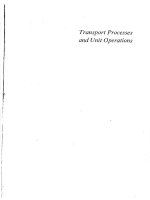
Let
us
consider another situation: a liquid at rest between
two
plates
(Figure
1-3).
At a given time the bottom plate moves with
a
velocity
V.
This
causes the fluid in its vicinity to also move. After
a
period of time with unsteady
flow we attain a linear velocity profile that is associated with steady-state flow.
At steady state
a
constant force
F
is needed.
In
this situation
0-v
- -
-p-

F
A
Y-0
-
where
p
is the fluid‘s viscosity (i.e., transport coefficient).
Lower plate
set
in motion
t=O
I
I
Velocity
buildup
I
Small
t
in
unsteady
,UAY,t)
I
flow
I
(1-7)
Figure 1-3.
mission from reference
I.
Copyright
1960,

John Wiley
and
Sons.)
Velocity profile development for steady laminar flow. (Adapted with per-
THE
TRANSPORT
COEFFICIENTS
5
Hence the
F/A
term is the flux of momentum (because force=
d(momentum)/dt. If we use the differential form (converting
FIA
to a shear
stress
r),
then we obtain
Units of
tyX
are poundals/ft2, dynes/cm2, and Newtons/m2.
This expression is known as Newton’s Law of Viscosity. Note that the shear
stress is subscripted with two letters. The reason for this is that momentum
transfer is not a vector (three components) but rather a tensor (nine components).
As
such, momentum transport, except for special cases, differs considerably
from heat transfer.
Finally, for the case
of
mass transfer because of concentration differences we
cite Fick’s First Law for a binary system:

where
JA,,
is the molar flux of component
A
in the
y
direction.
DAB,
the diffu-
sivity of
A
in
B
(the other component), is the applicable transport coefficient.
As
with Fourier’s Law, Fick’s First Law has three components and is a vec-
tor. Because of this there are many analogies between heat and mass transfer
as we will see later
in
the text. Units of the molar flux are lb moles/hr ft2,
g mole/sec cm2, and kg mole/sec m2.
THE TRANSPORT COEFFICIENTS
We have seen that the transport processes (momentum, heat, and mass) each
involve a property of the system (viscosity, thermal conductivity, diffusivity).
These properties are called the transport coefficients.
As
system properties they
are functions of temperature and pressure.
Expressions for the behavior of these properties in low-density gases can be
derived by using two approaches:

1.
The kinetic theory of gases
2.
Use of molecular interactions (Chapman-Enskog theory).
In
the first case the molecules are rigid, nonattracting, and spherical. They have
1.
A
mass
m
and a diameter
d
2.
A
concentration
n
(molecules/unit volume)
3.
A
distance of separation that is many times
d.
6
TRANSPORT PROCESSES AND TRANSPORT COEFFICIENTS
This approach gives the following expression for viscosity, thermal conduc-
tivity, and diffusivity:
where
K
is the Boltzmann constant.
(1-10)
where the gas is monatomic.

(1-1 1)
The subscripts
A
and
B
refer to gas
A
and gas
B.
If molecular interactions are considered (i.e., the molecules can both attract and
repel)
a
different set of relations are derived. This approach involves relating the
force of interaction,
F,
to the potential energy
4.
The latter quantity is represented
by
the Lennard-Jones (6-12) potential (see Figure 1-4)
(1-13)
where
n
is the collision diameter
(a
characteristic diameter) and
t
a characteristic
energy of interaction (see Table A-3-3 in Appendix for values of
CJ

and
e).
The Lennard-Jones potential predicts weak molecular attraction at great dis-
tances and ultimately strong repulsion
as
the molecules draw closer.
Resulting equations for viscosity, thermal conductivity, and diffusivity using
the Lennard-Jones potential are
rn
u=Qk
p
=
2.6693
x
10P-
(1-14)
where
p
is in units of kglm sec or pascal-seconds,
T
is
in
OK,
IJ
is in
A,
the
Qp
is
a

function of
KT/e
(see Appendix), and
M
is molecular weight.
(1-15)
where
k
is
in Wlm
OK,
u
is in
A,
and
Qk
=
Qp.
The expression is for
a
monatomic gas.
(1-16)
THE
TRANSPORT COEFFICIENTS
7
Molecules repel
one another at
cp(r,+
(sepfrations
r

crm
E
Molecules attract
I
one another at
I
separations
r >r,
I
I
I
When
r
=
3a,
I
lcpl
has dropped
off
to
less than
0.01
c
0
r*
-e
-

Figure
1-4.

from reference
1.
Copyright
1960,
John
Wiley and Sons.)
Lennard-Jones model potential energy function. (Adapted with permission
1
where
DAB
is units
of
m2/sec
P
is in atmospheres,
DAB
=
?(oA
+
oB),
CAB
=
m,
and
RDAB
is
a
function
of
KT/eAB (see Appendix

B,
Table A-3-4).
Example
1-1
is 7.6
x
man-Enskog approach.
The viscosity
of
isobutane
at
23°C and atmospheric pressure
pascal-sec. Compare this value to that calculated
by
the Chap-
From Table A-3-3
of
Appendix
A
we have
c
=
5.341
A,
EIK
=
313
K
Then,
K

TIE
=
296.1613 13
=
0.946 and from Table A-3-4
of
Appendix
B
we
obtain
Rp
=
1.634
m
D2Rp
p
=
2.6693
x
lop6-
p
=
2.6693
x
10-"
(58.12)(296.16)
(5.341)2( 1.634)
8
TRANSPORT PROCESSES AND TRANSPORT COEFFICIENTS
=

7.51
x
lop6
pascal-sec
%
error
=
[(7.6
-
7.51)/7.6]
x
100
=
1.18%
Example
1-2
and
14.7
psia.
Calculate the diffusivity for the methane-ethane system at
104°F
104+460
1.8
T=
K
=
313°K
Let methane be A and let ethane be
B.
Then.

=
0.0956
From Table
A
in the Appendix we have
(TA
=
3.822
A,
OB
=
4.418
A
&B
5
=
137"K,
-
=
230°K
K
K
DAB
=
~((TA
-
+
CJB)
=
i(3.822

+
4.418)
A
=
4.120
A
=
/(%)
(z)
=
J(137"K)(230"K)
=
177.5"K
K
KT
313
=
1.763
- -
____
EAB
177.5
From Table
A-3-4
in Appendix we have
QDAB
=
1.125
1.8583
x

1OP7J(3 13"K)'(0.0956)
(1)
(4.120)*(1.125)
DAB
=
DAB
=
1.66
x
m2/sec
The actual value is
1.84
x
lo-'
m2/sec. Percent error
is
9.7
percent.
TRANSPORT COEFFICIENT BEHAVIOR FOR HIGH DENSITY
GASES AND MIXTURES OF GASES
If gaseous systems have high densities, both the kinetic theory
of
gases and
the Chapman-Enskog theory fail to properly describe the transport coefficients'
behavior. Furthermore, the previously derived expression for viscosity and
TRANSPORT COEFFICIENT BEHAVIOR
9
10
Reduced temperature,
T,= T/T,

Figure
1-5.
(Courtesy
of
National Petroleum News.)
Reduced viscosity as a function of reduced pressure and temperature
(2).
thermal conductivity apply only to pure gases and not to gas mixtures. The
typical approach for such situations is
to
use the theory of corresponding states
as
a
method of dealing with the problem.
Figures
1-5,
1-6, 1-7, and 1-8 give correlation for viscosity and the thermal
conductivity
of
monatomic gases. One set (Figures 1-5 and 1-7) are plots of the
10
TRANSPORT PROCESSES AND TRANSPORT COEFFICIENTS
0.1
0.2
0.3
0.4
0.6 0.8
1
2
3

4
5
678910
20
Reduced pressure,
pr=
pIpc
Figure
1-6.
Modified reduced viscosity
as
a function
of
reduced temperature and pres-
sure
(3).
(Trans.
Am.
Inst. Mining, Metallurgical and Petroleum Engrs
201
1954
pp
264
ff;
N.
L.
Cam,
R.
Kobayashi,
D.B.

Burrows.)
reduced viscosity
(p/p(,
where
p(
is the viscosity at the critical point) or reduced
thermal conductivity
(klk,)
versus
(T/
T,),
reduced temperature, and
(plp,)
reduced pressure. The other set are plots
of
viscosity and thermal conductivity
divided by the values
(PO,
ko)
at atmospheric pressure and the same temperature.
TRANSPORT
COEFFICIENT
BEHAVIOR
11
10
9
8
7
6
5

4
3
9
32
X'
s
II
c
._
>
0
3
U
0
._
-
51
g
0.8
0.9
5
0.7
$
0.6
al
0.5
(r
0.4
Q,
U

3
U
0.2
0.2
0.1
0.3
0.4
0.6
0.8 1.0
2
3
4
5
6
78910
Reduced temperature,
Tr=
TIT,
Figure
1-7.
Reduced thermal conductivity (monatomic gases) as a function
of
reduced
temperature and pressure. (Reproduced with permission from reference
4.
Copyright
1957,
American Institute of Chemical Engineers.)
Values
of

pc
can
be
estimated from the empirical relations
(
M
T,)
kc
=
61.6
(C.)*/3
7.70
M'/2P,2/3
(Tc>'/6
Pc
=
(1-17)
(1-18)
12
TRANSPORT PROCESSES AND TRANSPORT COEFFICIENTS
10
a
6
.g
4
._
c
3
7J
83

1
Figure
1-8.
Modified reduced thermal conductivity as a function
of
reduced temperature
and pressure. (Reproduced with permission from reference
5.
Copyright
1953,
American
Institute
of
Chemical Engineers.)
h
where
p,
is in micropoises, T, is
in
OK,
P,
in atmospheres, and
V,
is in
cm'/g
mole.
The viscosity and thermal conductivity behavior of mixtures
of
gases at
low

densities is described semiempirically by the relations derived by Wilke
(6)
for
viscosity and by Mason and Saxena
(7)
for thermal conductivity:
(1-19)
(1-21)
j=1
TRANSPORT COEFFICIENT BEHAVIOR
13
The
@ij's
in equation (1-21) are given by equation (1-20). The
y's
refer to
For mixtures of dense gases the pseudocritical method is recommended. Here
the mole fractions of the components.
the critical properties for the mixture are given by
n
i=l
n
i=l
n
(1-22)
(1 -23)
(1 -24)
,=1
where
y,

is a mole fraction;
Pc,
,
Tc,, and
pc,
are pure component values. These
values are then used
to
determine the
PA
and
TA
values needed to obtain
(p/p,)
from Figure 1-5.
The same approach can be used for the thermal conductivity with Figure 1-7
if
k,
data are available or by using a
ko
value determined from equation (1-15).
Behavior of diffusivities is not as easily handled as the other transport coef-
ficients. The combination
(DAB
P)
is essentially a constant up to about 150 atm
pressure. Beyond that, the only available correlation is the one developed by
Slattery and Bird
(8).
This, however, should be used only with great caution

because it is based
on
very limited data
(8).
Example 1-3
40.3"C
using
Compare estimates
of
the viscosity of CO2 at 114.6 atm and
1. Figure 1-6 and an experimental viscosity value of 1800
x
lo-'
pascal-sec
2. The Chapman-Enskog relation and Figure 1-6.
for COz at 45.3 atm and 40.3"C
From Table
A-3-3
of Appendix
A,
T,
=
304.2"K and
P,
=
72.9 atmospheres.
For the first case we have
313.46 45.3
304.2 72.9
TR

=
-
=
1.03,
PR
=
-
=
0.622
so that
p'
=
1.12 and
p
1800
x
lo-' pascal-sec
Pu.#
1.12
Po=-=
=
1610
x
lo-' pascal-sec
For
P
=
114.6 atm we have
114.6
72.9

PR
=
~
=
1.57,
TR
=
1.03
14
TRANSPORT PROCESSES AND TRANSPORT COEFFICIENTS
so
that
p'
=
3.7 and
p
=
~'p.0
=
(3.7)(1610
x
lo-' pascals-sec)
=
6000
x
lo-' pascals-sec
For the second case, from Table A-3-3
of
Appendix we have
hi'

=
44.01,
(T
=
3.996
A,
Elk
=
190°K
and
KT
313.46
E
190
=
1.165

-
so
that from Table A-3-4
of
Appendix and
=
1.264 we obtain
m
(T=S2p
p
=
2.6693
x

(44.0
1)
(3 13.46)
p
=
2.6693
x
=
1553
x
lop8
pascal-sec
(3.
996)2
(
1.264)
From Figure 1-6,
p#
is still 3.7
so
that
p
=
(3.7)(1553
x
10
pascal-sec)
=
5746
x

lop8 pascal-sec
The actual experimental value is
5800
x
lopx pascal-sec. Percent errors for
case
1
and case 2 are 3.44% and 0.93%, respectively.
Example
1-4
02(y
=
0.039);
N2(y
=
0.828) at
1
atm and 293°K by using
Estimate the viscosity of
a
gas mixture of
C02(y
=
0.133);
I.
Figure
1-5
and the pseudocritical concept
2. Equations
(1

-19) and (1-20) with pure component viscosities of 1462,203
I,
and 1754
x
pascal-sec, respectively, for
C02,02,
and
N2.
In the first case the values of
T,,
P,
,
and
p,
(from Table A-3-3
of
Appendix)
are
as
follows:
T,
(i)
P,
(atmospheres)
p,
(pascal-seconds)
CO?
304.2 72.9
02
154.4 49.7

N2
126.2 33.5
3430
x
lo-'
2500
x
lo-'
1800
x
TRANSPORT COEFFICIENT BEHAVIOR
15
T,'
=
(0.133)(304.2"K)
+
(0.039)(154.4"K)
+
(0.828)(126.2"K)
T,!
=
150.97"K
P,'
=
[(0.133)(72.9)
+
(0.039)(49.7)
+
(0.828)(33.5)] atm
Pc!

=
39.37 atmospheres
P:.
=
[(0.133)(3430)
+
(0.039)(2500)
+
(0.828)(1800)
]
x
lo-'
pascal-sec
pt.
=
2044.1
x
lo-'
pascal-sec
Then
=
0.025
1
=
1.94,
P'
-
-
293
T'

-
-
-
150.97
-
39.37
From Figure 1-5 we have
P
=
(0.855)(2044.1
x
lo-'
pascal-sec)
=
1747.7
x
lo-' pascal-sec
For case 2, let
C02
=
1,02
=
2, and
N2
=
3. Then:
1
1
1
.oo

2 1.38
3 1.57
2
1
0.73
2
1
.oo
3 1.14
3
I
0.64
2
0.88
3
1
.oo
1
.oo
0.72
0.83
1.39
1
.oo
1.16
1.20
0.86
1
.oo
1

.oo
0.73
0.73
1.39
1
.oo
1.04
1.37
0.94
1
.oo
j=1
(0.133)(1462) (0.039)(203
1)
(0.828)(
1754)
]
(1.06)
(1.05)
+
Pmix
=
+
x
lo-'
pascal-sec
pmix
=
1714
x

lo-'
pascal-sec
16
TRANSPORT PROCESSES AND TRANSPORT COEFFICIENTS
Actual experimental value of the mixture viscosity is 1793
x
lop8
pascal-sec.
The percent errors are 2.51 and
4.41%,
respectively, for cases
1
and
2.
TRANSPORT COEFFICIENTS IN LIQUID AND SOLID SYSTEMS
In general, the understanding of the behavior of transport coefficients in gases
is far greater than that for liquid systems. This can be partially explained by
seeing that liquids are much more dense than gases. Additionally, theoretical and
experimental work for gases is far more voluminous than for liquids. In any case
the
net
result is that approaches to transport coefficient behavior in liquid systems
are mainly empirical
in
nature.
An approach used for liquid viscosities is based on an application of the Eyring
(9,10)
activated rate theory. This yields an expression of the form
Nh
V

(
1-25)
where
N
is Avogadro’s number,
h
is Plancks constant,
V
is the molar volume,
and
AU,,,
is the molar internal energy change at the liquid’s normal boiling
point.
The Eyring equation is at best an approximation; thus
it
is recommended that
liquid viscosities be estimated using the nomograph given
in
Figure
B-1
of the
appendix.
For thermal conductivity the theory of Bridgman
(I
1) yielded
k
=
2.80
(
;)*I3

KVs
where
V,
the sonic velocity, is
(1
-26)
(
1-27)
The foregoing expressions for both viscosity and thermal conductivity are for
pures. For mixtures
it
is recommended that the pseudocritical method be used
where possible with liquid regions of Figures 1-5 through 1-8.
Diffusivities in liquids can be treated by the Stokes-Einstein equation
(1-28)
where
RA
is the diffusing species radius and
p~
is the solvent viscosity.