TECHNICAL ENGLISH I&II
Bạn đang xem bản rút gọn của tài liệu. Xem và tải ngay bản đầy đủ của tài liệu tại đây (18.54 MB, 153 trang )
Harran University
Engineering Faculty
Department of Mechanical Engineering
Reading Texts For Mechanical
Engineering
Technical English I & II
Prepared by
Assoc. Prof. Dr. Hüsamettin BULUT
October-2006
Şanlıurfa
Content
¾ Fluid Dynamics
¾ Heat Transfer
¾ Fuels
¾ Energy Sources (Solar, Wind and Geothermal Energy)
¾ Air-Conditioning
¾ Heat Exchangers
¾ HVAC Equipments and Systems
¾ Manufacturing and Systems
¾ Materials
¾ Dynamics
¾ Vibrations
¾ Pressure Vessels
¾ Steam and Power Systems
¾ Engineering Thermodynamics
¾ Turbomachinery
¾ Specifications and Catalogs for Some Machines and Systems
1.1 Preliminary Remarks
Fluid mechanics is the study of fluids either in motion (fluid dynamics) or at rest (fluid
statics) and the subsequent effects of the fluid upon the boundaries, which may be ei-
ther solid surfaces or interfaces with other fluids. Both gases and liquids are classified
as fluids, and the number of fluids engineering applications is enormous: breathing,
blood flow, swimming, pumps, fans, turbines, airplanes, ships, rivers, windmills, pipes,
missiles, icebergs, engines, filters, jets, and sprinklers, to name a few. When you think
about it, almost everything on this planet either is a fluid or moves within or near a
fluid.
The essence of the subject of fluid flow is a judicious compromise between theory
and experiment. Since fluid flow is a branch of mechanics, it satisfies a set of well-
documented basic laws, and thus a great deal of theoretical treatment is available. How-
ever, the theory is often frustrating, because it applies mainly to idealized situations
which may be invalid in practical problems. The two chief obstacles to a workable the-
ory are geometry and viscosity. The basic equations of fluid motion (Chap. 4) are too
difficult to enable the analyst to attack arbitrary geometric configurations. Thus most
textbooks concentrate on flat plates, circular pipes, and other easy geometries. It is pos-
sible to apply numerical computer techniques to complex geometries, and specialized
textbooks are now available to explain the new computational fluid dynamics (CFD)
approximations and methods [1, 2, 29].
1
This book will present many theoretical re-
sults while keeping their limitations in mind.
The second obstacle to a workable theory is the action of viscosity, which can be
neglected only in certain idealized flows (Chap. 8). First, viscosity increases the diffi-
culty of the basic equations, although the boundary-layer approximation found by Lud-
wig Prandtl in 1904 (Chap. 7) has greatly simplified viscous-flow analyses. Second,
viscosity has a destabilizing effect on all fluids, giving rise, at frustratingly small ve-
locities, to a disorderly, random phenomenon called turbulence. The theory of turbu-
lent flow is crude and heavily backed up by experiment (Chap. 6), yet it can be quite
serviceable as an engineering estimate. Textbooks now present digital-computer tech-
niques for turbulent-flow analysis [32], but they are based strictly upon empirical as-
sumptions regarding the time mean of the turbulent stress field.
Chapter 1
Introduction
3
1
Numbered references appear at the end of each chapter.
| | | |
▲
▲
e-Text Main Menu
Textbook Table of Contents
Study Guide
1.2 The Concept of a Fluid
Thus there is theory available for fluid-flow problems, but in all cases it should be
backed up by experiment. Often the experimental data provide the main source of in-
formation about specific flows, such as the drag and lift of immersed bodies (Chap. 7).
Fortunately, fluid mechanics is a highly visual subject, with good instrumentation [4,
5, 35], and the use of dimensional analysis and modeling concepts (Chap. 5) is wide-
spread. Thus experimentation provides a natural and easy complement to the theory.
You should keep in mind that theory and experiment should go hand in hand in all
studies of fluid mechanics.
From the point of view of fluid mechanics, all matter consists of only two states, fluid
and solid. The difference between the two is perfectly obvious to the layperson, and it
is an interesting exercise to ask a layperson to put this difference into words. The tech-
nical distinction lies with the reaction of the two to an applied shear or tangential stress.
A solid can resist a shear stress by a static deformation; a fluid cannot. Any shear
stress applied to a fluid, no matter how small, will result in motion of that fluid. The
fluid moves and deforms continuously as long as the shear stress is applied. As a corol-
lary, we can say that a fluid at rest must be in a state of zero shear stress, a state of-
ten called the hydrostatic stress condition in structural analysis. In this condition, Mohr’s
circle for stress reduces to a point, and there is no shear stress on any plane cut through
the element under stress.
Given the definition of a fluid above, every layperson also knows that there are two
classes of fluids, liquids and gases. Again the distinction is a technical one concerning
the effect of cohesive forces. A liquid, being composed of relatively close-packed mol-
ecules with strong cohesive forces, tends to retain its volume and will form a free sur-
face in a gravitational field if unconfined from above. Free-surface flows are domi-
nated by gravitational effects and are studied in Chaps. 5 and 10. Since gas molecules
are widely spaced with negligible cohesive forces, a gas is free to expand until it en-
counters confining walls. A gas has no definite volume, and when left to itself with-
out confinement, a gas forms an atmosphere which is essentially hydrostatic. The hy-
drostatic behavior of liquids and gases is taken up in Chap. 2. Gases cannot form a
free surface, and thus gas flows are rarely concerned with gravitational effects other
than buoyancy.
Figure 1.1 illustrates a solid block resting on a rigid plane and stressed by its own
weight. The solid sags into a static deflection, shown as a highly exaggerated dashed
line, resisting shear without flow. A free-body diagram of element A on the side of the
block shows that there is shear in the block along a plane cut at an angle
through A.
Since the block sides are unsupported, element A has zero stress on the left and right
sides and compression stress
ϭϪp on the top and bottom. Mohr’s circle does not
reduce to a point, and there is nonzero shear stress in the block.
By contrast, the liquid and gas at rest in Fig. 1.1 require the supporting walls in or-
der to eliminate shear stress. The walls exert a compression stress of Ϫp and reduce
Mohr’s circle to a point with zero shear everywhere, i.e., the hydrostatic condition. The
liquid retains its volume and forms a free surface in the container. If the walls are re-
moved, shear develops in the liquid and a big splash results. If the container is tilted,
shear again develops, waves form, and the free surface seeks a horizontal configura-
4 Chapter 1 Introduction
| | | |
▲
▲
e-Text Main Menu
Textbook Table of Contents
Study Guide
tion, pouring out over the lip if necessary. Meanwhile, the gas is unrestrained and ex-
pands out of the container, filling all available space. Element A in the gas is also hy-
drostatic and exerts a compression stress Ϫp on the walls.
In the above discussion, clear decisions could be made about solids, liquids, and
gases. Most engineering fluid-mechanics problems deal with these clear cases, i.e., the
common liquids, such as water, oil, mercury, gasoline, and alcohol, and the common
gases, such as air, helium, hydrogen, and steam, in their common temperature and pres-
sure ranges. There are many borderline cases, however, of which you should be aware.
Some apparently “solid” substances such as asphalt and lead resist shear stress for short
periods but actually deform slowly and exhibit definite fluid behavior over long peri-
ods. Other substances, notably colloid and slurry mixtures, resist small shear stresses
but “yield” at large stress and begin to flow as fluids do. Specialized textbooks are de-
voted to this study of more general deformation and flow, a field called rheology [6].
Also, liquids and gases can coexist in two-phase mixtures, such as steam-water mix-
tures or water with entrapped air bubbles. Specialized textbooks present the analysis
1.2 The Concept of a Fluid 5
Static
deflection
Free
surface
Hydrostatic
condition
Liquid
Solid
A
AA
(a) (c)
(b) (d)
0
0
AA
Gas
(1)
– p – p
p
p
p
= 0
τ
θ
θ
θ
2
1
– = p – = p
σ
σ
1
τ
σ
τ
σ
τ
σ
Fig. 1.1 A solid at rest can resist
shear. (a) Static deflection of the
solid; (b) equilibrium and Mohr’s
circle for solid element A. A fluid
cannot resist shear. (c) Containing
walls are needed; (d) equilibrium
and Mohr’s circle for fluid
element A.
| | | |
▲
▲
e-Text Main Menu
Textbook Table of Contents
Study Guide
1.4 Dimensions and Units
above which aggregate variations may be important. The density
of a fluid is best
defined as
ϭ lim
␦
ᐂ→
␦
ᐂ*
ᎏ
␦
␦
ᐂ
m
ᎏ
(1.1)
The limiting volume
␦
ᐂ* is about 10
Ϫ9
mm
3
for all liquids and for gases at atmospheric
pressure. For example, 10
Ϫ9
mm
3
of air at standard conditions contains approximately
3 ϫ 10
7
molecules, which is sufficient to define a nearly constant density according to
Eq. (1.1). Most engineering problems are concerned with physical dimensions much larger
than this limiting volume, so that density is essentially a point function and fluid proper-
ties can be thought of as varying continually in space, as sketched in Fig. 1.2a. Such a
fluid is called a continuum, which simply means that its variation in properties is so smooth
that the differential calculus can be used to analyze the substance. We shall assume that
continuum calculus is valid for all the analyses in this book. Again there are borderline
cases for gases at such low pressures that molecular spacing and mean free path
3
are com-
parable to, or larger than, the physical size of the system. This requires that the contin-
uum approximation be dropped in favor of a molecular theory of rarefied-gas flow [8]. In
principle, all fluid-mechanics problems can be attacked from the molecular viewpoint, but
no such attempt will be made here. Note that the use of continuum calculus does not pre-
clude the possibility of discontinuous jumps in fluid properties across a free surface or
fluid interface or across a shock wave in a compressible fluid (Chap. 9). Our calculus in
Chap. 4 must be flexible enough to handle discontinuous boundary conditions.
A dimension is the measure by which a physical variable is expressed quantitatively.
A unit is a particular way of attaching a number to the quantitative dimension. Thus
length is a dimension associated with such variables as distance, displacement, width,
deflection, and height, while centimeters and inches are both numerical units for ex-
pressing length. Dimension is a powerful concept about which a splendid tool called
dimensional analysis has been developed (Chap. 5), while units are the nitty-gritty, the
number which the customer wants as the final answer.
Systems of units have always varied widely from country to country, even after in-
ternational agreements have been reached. Engineers need numbers and therefore unit
systems, and the numbers must be accurate because the safety of the public is at stake.
You cannot design and build a piping system whose diameter is D and whose length
is L. And U.S. engineers have persisted too long in clinging to British systems of units.
There is too much margin for error in most British systems, and many an engineering
student has flunked a test because of a missing or improper conversion factor of 12 or
144 or 32.2 or 60 or 1.8. Practicing engineers can make the same errors. The writer is
aware from personal experience of a serious preliminary error in the design of an air-
craft due to a missing factor of 32.2 to convert pounds of mass to slugs.
In 1872 an international meeting in France proposed a treaty called the Metric Con-
vention, which was signed in 1875 by 17 countries including the United States. It was
an improvement over British systems because its use of base 10 is the foundation of
our number system, learned from childhood by all. Problems still remained because
1.4 Dimensions and Units 7
3
The mean distance traveled by molecules between collisions.
| | | |
▲
▲
e-Text Main Menu
Textbook Table of Contents
Study Guide
even the metric countries differed in their use of kiloponds instead of dynes or new-
tons, kilograms instead of grams, or calories instead of joules. To standardize the met-
ric system, a General Conference of Weights and Measures attended in 1960 by 40
countries proposed the International System of Units (SI). We are now undergoing a
painful period of transition to SI, an adjustment which may take many more years to
complete. The professional societies have led the way. Since July 1, 1974, SI units have
been required by all papers published by the American Society of Mechanical Engi-
neers, which prepared a useful booklet explaining the SI [9]. The present text will use
SI units together with British gravitational (BG) units.
In fluid mechanics there are only four primary dimensions from which all other dimen-
sions can be derived: mass, length, time, and temperature.
4
These dimensions and their units
in both systems are given in Table 1.1. Note that the kelvin unit uses no degree symbol.
The braces around a symbol like {M} mean “the dimension” of mass. All other variables
in fluid mechanics can be expressed in terms of {M}, {L}, {T}, and {⌰}. For example, ac-
celeration has the dimensions {LT
Ϫ2
}. The most crucial of these secondary dimensions is
force, which is directly related to mass, length, and time by Newton’s second law
F ϭ ma (1.2)
From this we see that, dimensionally, {F} ϭ {MLT
Ϫ2
}. A constant of proportionality
is avoided by defining the force unit exactly in terms of the primary units. Thus we
define the newton and the pound of force
1 newton of force ϭ 1 N ϵ 1 kg и m/s
2
(1.3)
1 pound of force ϭ 1 lbf ϵ 1 slug и ft/s
2
ϭ 4.4482 N
In this book the abbreviation lbf is used for pound-force and lb for pound-mass. If in-
stead one adopts other force units such as the dyne or the poundal or kilopond or adopts
other mass units such as the gram or pound-mass, a constant of proportionality called
g
c
must be included in Eq. (1.2). We shall not use g
c
in this book since it is not nec-
essary in the SI and BG systems.
A list of some important secondary variables in fluid mechanics, with dimensions
derived as combinations of the four primary dimensions, is given in Table 1.2. A more
complete list of conversion factors is given in App. C.
8 Chapter 1 Introduction
4
If electromagnetic effects are important, a fifth primary dimension must be included, electric current
{I}, whose SI unit is the ampere (A).
Primary dimension SI unit BG unit Conversion factor
Mass {M} Kilogram (kg) Slug 1 slug ϭ 14.5939 kg
Length {L} Meter (m) Foot (ft) 1 ft ϭ 0.3048 m
Time {T} Second (s) Second (s) 1 s ϭ 1 s
Temperature {⌰} Kelvin (K) Rankine (°R) 1 K ϭ 1.8°R
Table 1.1 Primary Dimensions in
SI and BG Systems
Primary Dimensions
| | | |
▲
▲
e-Text Main Menu
Textbook Table of Contents
Study Guide
Part (a)
Part (b)
Part (c)
EXAMPLE 1.1
A body weighs 1000 lbf when exposed to a standard earth gravity g ϭ 32.174 ft/s
2
. (a) What is
its mass in kg? (b) What will the weight of this body be in N if it is exposed to the moon’s stan-
dard acceleration g
moon
ϭ 1.62 m/s
2
? (c) How fast will the body accelerate if a net force of 400
lbf is applied to it on the moon or on the earth?
Solution
Equation (1.2) holds with F ϭ weight and a ϭ g
earth
:
F ϭ W ϭ mg ϭ 1000 lbf ϭ (m slugs)(32.174 ft/s
2
)
or
m ϭ
ᎏ
3
1
2
0
.1
0
7
0
4
ᎏ
ϭ (31.08 slugs)(14.5939 kg/slug) ϭ 453.6 kg Ans. (a)
The change from 31.08 slugs to 453.6 kg illustrates the proper use of the conversion factor
14.5939 kg/slug.
The mass of the body remains 453.6 kg regardless of its location. Equation (1.2) applies with a
new value of a and hence a new force
F ϭ W
moon
ϭ mg
moon
ϭ (453.6 kg)(1.62 m/s
2
) ϭ 735 N Ans. (b)
This problem does not involve weight or gravity or position and is simply a direct application
of Newton’s law with an unbalanced force:
F ϭ 400 lbf ϭ ma ϭ (31.08 slugs)(a ft/s
2
)
or
a ϭ
ᎏ
3
4
1
0
.0
0
8
ᎏ
ϭ 12.43 ft/s
2
ϭ 3.79 m/s
2
Ans. (c)
This acceleration would be the same on the moon or earth or anywhere.
1.4 Dimensions and Units 9
Secondary dimension SI unit BG unit Conversion factor
Area {L
2
}m
2
ft
2
1 m
2
ϭ 10.764 ft
2
Volume {L
3
}m
3
ft
3
1 m
3
ϭ 35.315 ft
3
Velocity {LT
Ϫ1
} m/s ft/s 1 ft/s ϭ 0.3048 m/s
Acceleration {LT
Ϫ2
} m/s
2
ft/s
2
1 ft/s
2
ϭ 0.3048 m/s
2
Pressure or stress
{ML
Ϫ1
T
Ϫ2
}Paϭ N/m
2
lbf/ft
2
1 lbf/ft
2
ϭ 47.88 Pa
Angular velocity {T
Ϫ1
}s
Ϫ1
s
Ϫ1
1 s
Ϫ1
ϭ 1 s
Ϫ1
Energy, heat, work
{ML
2
T
Ϫ2
}Jϭ N и mftи lbf 1 ft и lbf ϭ 1.3558 J
Power {ML
2
T
Ϫ3
}Wϭ J/s ft и lbf/s 1 ft и lbf/s ϭ 1.3558 W
Density {ML
Ϫ3
} kg/m
3
slugs/ft
3
1 slug/ft
3
ϭ 515.4 kg/m
3
Viscosity {ML
Ϫ1
T
Ϫ1
} kg/(m и s) slugs/(ft и s) 1 slug/(ft и s) ϭ 47.88 kg/(m и s)
Specific heat {L
2
T
Ϫ2
⌰
Ϫ1
}m
2
/(s
2
и K) ft
2
/(s
2
и °R) 1 m
2
/(s
2
и K) ϭ 5.980 ft
2
/(s
2
и °R)
Table 1.2 Secondary Dimensions in
Fluid Mechanics
| | | |
▲
▲
e-Text Main Menu
Textbook Table of Contents
Study Guide
Convenient Prefixes in
Powers of 10
Part (a)
Part (b)
Meanwhile, we conclude that dimensionally inconsistent equations, though they
abound in engineering practice, are misleading and vague and even dangerous, in the
sense that they are often misused outside their range of applicability.
Engineering results often are too small or too large for the common units, with too
many zeros one way or the other. For example, to write p ϭ 114,000,000 Pa is long
and awkward. Using the prefix “M” to mean 10
6
, we convert this to a concise p ϭ
114 MPa (megapascals). Similarly, t ϭ 0.000000003 s is a proofreader’s nightmare
compared to the equivalent t ϭ 3 ns (nanoseconds). Such prefixes are common and
convenient, in both the SI and BG systems. A complete list is given in Table 1.3.
EXAMPLE 1.4
In 1890 Robert Manning, an Irish engineer, proposed the following empirical formula for the
average velocity V in uniform flow due to gravity down an open channel (BG units):
V ϭ
ᎏ
1.
n
49
ᎏ
R
2/3
S
1/2
(1)
where R ϭ hydraulic radius of channel (Chaps. 6 and 10)
S ϭ channel slope (tangent of angle that bottom makes with horizontal)
n ϭ Manning’s roughness factor (Chap. 10)
and n is a constant for a given surface condition for the walls and bottom of the channel. (a)Is
Manning’s formula dimensionally consistent? (b) Equation (1) is commonly taken to be valid in
BG units with n taken as dimensionless. Rewrite it in SI form.
Solution
Introduce dimensions for each term. The slope S, being a tangent or ratio, is dimensionless, de-
noted by {unity} or {1}. Equation (1) in dimensional form is
Ά
ᎏ
T
L
ᎏ
·
ϭ
Ά
ᎏ
1.
n
49
ᎏ
·
{L
2/3
}{1}
This formula cannot be consistent unless {1.49/n} ϭ {L
1/3
/T}. If n is dimensionless (and it is
never listed with units in textbooks), then the numerical value 1.49 must have units. This can be
tragic to an engineer working in a different unit system unless the discrepancy is properly doc-
umented. In fact, Manning’s formula, though popular, is inconsistent both dimensionally and
physically and does not properly account for channel-roughness effects except in a narrow range
of parameters, for water only.
From part (a), the number 1.49 must have dimensions {L
1/3
/T} and thus in BG units equals
1.49 ft
1/3
/s. By using the SI conversion factor for length we have
(1.49 ft
1/3
/s)(0.3048 m/ft)
1/3
ϭ 1.00 m
1/3
/s
Therefore Manning’s formula in SI becomes
V ϭ
ᎏ
1
n
.0
ᎏ
R
2/3
S
1/2
Ans. (b) (2)
1.4 Dimensions and Units 13
Table 1.3 Convenient Prefixes
for Engineering Units
Multiplicative
factor Prefix Symbol
10
12
tera T
10
9
giga G
10
6
mega M
10
3
kilo k
10
2
hecto h
10 deka da
10
Ϫ1
deci d
10
Ϫ2
centi c
10
Ϫ3
milli m
10
Ϫ6
micro
10
Ϫ9
nano n
10
Ϫ12
pico p
10
Ϫ15
femto f
10
Ϫ18
atto a
| | | |
▲
▲
e-Text Main Menu
Textbook Table of Contents
Study Guide
1.6 Thermodynamic Properties
of a Fluid
the acceleration of gravity. In the limit as ⌬x and ⌬t become very small, the above estimate re-
duces to a partial-derivative expression for convective x-acceleration:
a
x,convective
ϭ lim
⌬t
→
0
ᎏ
⌬
⌬
u
t
ᎏ
ϭ u
ᎏ
Ѩ
Ѩ
u
x
ᎏ
In three-dimensional flow (Sec. 4.1) there are nine of these convective terms.
While the velocity field V is the most important fluid property, it interacts closely with
the thermodynamic properties of the fluid. We have already introduced into the dis-
cussion the three most common such properties
1. Pressure p
2. Density
3. Temperature T
These three are constant companions of the velocity vector in flow analyses. Four other
thermodynamic properties become important when work, heat, and energy balances are
treated (Chaps. 3 and 4):
4. Internal energy e
5. Enthalpy h ϭ û ϩ p/
6. Entropy s
7. Specific heats c
p
and c
v
In addition, friction and heat conduction effects are governed by the two so-called trans-
port properties:
8. Coefficient of viscosity
9. Thermal conductivity k
All nine of these quantities are true thermodynamic properties which are determined
by the thermodynamic condition or state of the fluid. For example, for a single-phase
substance such as water or oxygen, two basic properties such as pressure and temper-
ature are sufficient to fix the value of all the others:
ϭ
(p, T ) h ϭ h(p, T)
ϭ
(p, T ) (1.5)
and so on for every quantity in the list. Note that the specific volume, so important in
thermodynamic analyses, is omitted here in favor of its inverse, the density
.
Recall that thermodynamic properties describe the state of a system, i.e., a collec-
tion of matter of fixed identity which interacts with its surroundings. In most cases
here the system will be a small fluid element, and all properties will be assumed to be
continuum properties of the flow field:
ϭ
(x, y, z, t), etc.
Recall also that thermodynamics is normally concerned with static systems, whereas
fluids are usually in variable motion with constantly changing properties. Do the prop-
erties retain their meaning in a fluid flow which is technically not in equilibrium? The
answer is yes, from a statistical argument. In gases at normal pressure (and even more
so for liquids), an enormous number of molecular collisions occur over a very short
distance of the order of 1
m, so that a fluid subjected to sudden changes rapidly ad-
16 Chapter 1 Introduction
| | | |
▲
▲
e-Text Main Menu
Textbook Table of Contents
Study Guide
Temperature
Specific Weight
Density
justs itself toward equilibrium. We therefore assume that all the thermodynamic prop-
erties listed above exist as point functions in a flowing fluid and follow all the laws
and state relations of ordinary equilibrium thermodynamics. There are, of course, im-
portant nonequilibrium effects such as chemical and nuclear reactions in flowing flu-
ids which are not treated in this text.
Pressure is the (compression) stress at a point in a static fluid (Fig. 1.1). Next to ve-
locity, the pressure p is the most dynamic variable in fluid mechanics. Differences or
gradients in pressure often drive a fluid flow, especially in ducts. In low-speed flows,
the actual magnitude of the pressure is often not important, unless it drops so low as to
cause vapor bubbles to form in a liquid. For convenience, we set many such problem
assignments at the level of 1 atm ϭ 2116 lbf/ft
2
ϭ 101,300 Pa. High-speed (compressible)
gas flows (Chap. 9), however, are indeed sensitive to the magnitude of pressure.
Temperature T is a measure of the internal energy level of a fluid. It may vary con-
siderably during high-speed flow of a gas (Chap. 9). Although engineers often use Cel-
sius or Fahrenheit scales for convenience, many applications in this text require ab-
solute (Kelvin or Rankine) temperature scales:
°R ϭ °F ϩ 459.69
K ϭ °C ϩ 273.16
If temperature differences are strong, heat transfer may be important [10], but our con-
cern here is mainly with dynamic effects. We examine heat-transfer principles briefly
in Secs. 4.5 and 9.8.
The density of a fluid, denoted by
(lowercase Greek rho), is its mass per unit vol-
ume. Density is highly variable in gases and increases nearly proportionally to the pres-
sure level. Density in liquids is nearly constant; the density of water (about 1000 kg/m
3
)
increases only 1 percent if the pressure is increased by a factor of 220. Thus most liq-
uid flows are treated analytically as nearly “incompressible.”
In general, liquids are about three orders of magnitude more dense than gases at at-
mospheric pressure. The heaviest common liquid is mercury, and the lightest gas is hy-
drogen. Compare their densities at 20°C and 1 atm:
Mercury:
ϭ 13,580 kg/m
3
Hydrogen:
ϭ 0.0838 kg/m
3
They differ by a factor of 162,000! Thus the physical parameters in various liquid and
gas flows might vary considerably. The differences are often resolved by the use of di-
mensional analysis (Chap. 5). Other fluid densities are listed in Tables A.3 and A.4 (in
App. A).
The specific weight of a fluid, denoted by
␥
(lowercase Greek gamma), is its weight
per unit volume. Just as a mass has a weight W ϭ mg, density and specific weight are
simply related by gravity:
␥
ϭ
g (1.6)
1.6 Thermodynamic Properties of a Fluid 17
Pressure
| | | |
▲
▲
e-Text Main Menu
Textbook Table of Contents
Study Guide
Specific Gravity
Potential and Kinetic Energies
The units of
␥
are weight per unit volume, in lbf/ft
3
or N/m
3
. In standard earth grav-
ity, g ϭ 32.174 ft/s
2
ϭ 9.807 m/s
2
. Thus, e.g., the specific weights of air and water at
20°C and 1 atm are approximately
␥
air
ϭ (1.205 kg/m
3
)(9.807 m/s
2
) ϭ 11.8 N/m
3
ϭ 0.0752 lbf/ft
3
␥
water
ϭ (998 kg/m
3
)(9.807 m/s
2
) ϭ 9790 N/m
3
ϭ 62.4 lbf/ft
3
Specific weight is very useful in the hydrostatic-pressure applications of Chap. 2. Spe-
cific weights of other fluids are given in Tables A.3 and A.4.
Specific gravity, denoted by SG, is the ratio of a fluid density to a standard reference
fluid, water (for liquids), and air (for gases):
SG
gas
ϭ
ᎏ
g
a
a
ir
s
ᎏ
ϭ
ᎏ
1.20
5
g
k
as
g/m
3
ᎏ
(1.7)
SG
liquid
ϭ
ᎏ
l
w
iq
a
u
te
id
r
ᎏ
ϭ
ᎏ
99
8
li
k
qu
g
i
/
d
m
3
ᎏ
For example, the specific gravity of mercury (Hg) is SG
Hg
ϭ 13,580/998 Ϸ 13.6. En-
gineers find these dimensionless ratios easier to remember than the actual numerical
values of density of a variety of fluids.
In thermostatics the only energy in a substance is that stored in a system by molecu-
lar activity and molecular bonding forces. This is commonly denoted as internal en-
ergy û. A commonly accepted adjustment to this static situation for fluid flow is to add
two more energy terms which arise from newtonian mechanics: the potential energy
and kinetic energy.
The potential energy equals the work required to move the system of mass m from
the origin to a position vector r ϭ ix ϩ jy ϩ kz against a gravity field g. Its value is
Ϫmg ؒ r, or Ϫg ؒ r per unit mass. The kinetic energy equals the work required to change
the speed of the mass from zero to velocity V. Its value is
ᎏ
1
2
ᎏ
mV
2
or
ᎏ
1
2
ᎏ
V
2
per unit mass.
Then by common convention the total stored energy e per unit mass in fluid mechan-
ics is the sum of three terms:
e ϭ û ϩ
ᎏ
1
2
ᎏ
V
2
ϩ (Ϫg ؒ r) (1.8)
Also, throughout this book we shall define z as upward, so that g ϭϪgk and g ؒ r ϭ
Ϫgz. Then Eq. (1.8) becomes
e ϭ û ϩ
ᎏ
1
2
ᎏ
V
2
ϩ gz (1.9)
The molecular internal energy û is a function of T and p for the single-phase pure sub-
stance, whereas the potential and kinetic energies are kinematic properties.
Thermodynamic properties are found both theoretically and experimentally to be re-
lated to each other by state relations which differ for each substance. As mentioned,
18 Chapter 1 Introduction
State Relations for Gases
| | | |
▲
▲
e-Text Main Menu
Textbook Table of Contents
Study Guide
we shall confine ourselves here to single-phase pure substances, e.g., water in its liq-
uid phase. The second most common fluid, air, is a mixture of gases, but since the mix-
ture ratios remain nearly constant between 160 and 2200 K, in this temperature range
air can be considered to be a pure substance.
All gases at high temperatures and low pressures (relative to their critical point) are
in good agreement with the perfect-gas law
p ϭ
RT R ϭ c
p
Ϫ
c
v
ϭ gas constant (1.10)
Since Eq. (1.10) is dimensionally consistent, R has the same dimensions as specific
heat, {L
2
T
Ϫ2
⌰
Ϫ1
}, or velocity squared per temperature unit (kelvin or degree Rank-
ine). Each gas has its own constant R, equal to a universal constant ⌳ divided by the
molecular weight
R
gas
ϭ
ᎏ
M
⌳
gas
ᎏ
(1.11)
where ⌳ϭ49,700 ft
2
/(s
2
и °R) ϭ 8314 m
2
/(s
2
и K). Most applications in this book are
for air, with M ϭ 28.97:
R
air
ϭ 1717 ft
2
/(s
2
и °R) ϭ 287 m
2
/(s
2
и K) (1.12)
Standard atmospheric pressure is 2116 lbf/ft
2
, and standard temperature is 60°F ϭ
520°R. Thus standard air density is
air
ϭ
ᎏ
(171
2
7
1
)
1
(
6
520)
ᎏ
ϭ 0.00237 slug/ft
3
ϭ 1.22 kg/m
3
(1.13)
This is a nominal value suitable for problems.
One proves in thermodynamics that Eq. (1.10) requires that the internal molecular
energy û of a perfect gas vary only with temperature: û ϭ û(T). Therefore the specific
heat c
v
also varies only with temperature:
c
v
ϭ
ᎏ
Ѩ
Ѩ
T
û
ᎏ
ϭ
ᎏ
d
d
T
û
ᎏ
ϭ c
v
(T)
or dû ϭ c
v
(T) dT (1.14)
In like manner h and c
p
of a perfect gas also vary only with temperature:
h ϭ û ϩ
ᎏ
p
ᎏ
ϭ û ϩ RT ϭ h(T)
c
p
ϭ
ᎏ
Ѩ
Ѩ
T
h
ᎏ
p
ϭ
ᎏ
d
d
T
h
ᎏ
ϭ c
p
(T) (1.15)
dh ϭ c
p
(T) dT
The ratio of specific heats of a perfect gas is an important dimensionless parameter in
compressible-flow analysis (Chap. 9)
k ϭ
ᎏ
c
c
p
v
ᎏ
ϭ k(T) Ն 1 (1.16)
1.6 Thermodynamic Properties of a Fluid 19
| | | |
▲
▲
e-Text Main Menu
Textbook Table of Contents
Study Guide
10 Introduction §1.3
The term in parentheses is positive, so
˙
S
Un
> 0. This agrees with Clau-
sius’s statement of the Second Law of Thermodynamics.
Notice an odd fact here: The rate of heat transfer, Q, and hence
˙
S
Un
,
is determined by the wall’s resistance to heat flow. Although the wall
is the agent that causes the entropy of the universe to increase, its own
entropy does not changes. Only the entropies of the reservoirs change.
1.3 Modes of heat transfer
Figure 1.3 shows an analogy that might be useful in fixing the concepts
of heat conduction, convection, and radiation as we proceed to look at
each in some detail.
Heat conduction
Fourier’s law. Joseph Fourier (see Fig. 1.4) published his remarkable
book Théorie Analytique de la Chaleurin 1822. In it he formulated a very
complete exposition of the theory of heat conduction.
Hebegan his treatise by stating the empirical law that bears his name:
the heat flux,
3
q (W/m
2
), resulting from thermal conduction is proportional
to the magnitude of the temperature gradient and opposite to it in sign.If
we call the constant of proportionality, k, then
q =−k
dT
dx
(1.8)
The constant, k, is called the thermal conductivity. It obviously must have
the dimensions W/m·K, or J/m·s·K, or Btu/h·ft·
◦
F if eqn. (1.8)istobe
dimensionally correct.
The heat flux is a vector quantity. Equation (1.8) tells us that if temper-
ature decreases with x, q will be positive—it will flow in the x-direction.
If T increases with x, q will be negative—it will flow opposite the x-
direction. In either case, q will flow from higher temperatures to lower
temperatures. Equation (1.8) is the one-dimensional form of Fourier’s
law. We develop its three-dimensional form in Chapter 2, namely:
q =−k ∇T
3
The heat flux, q, is a heat rate per unit area and can be expressed as Q/A, where A
is an appropriate area.
Figure 1.3 An analogy for the three modes of heat transfer.
11
§1.3 Modes of heat transfer 13
Example 1.1
The front of a slab of lead (k = 35 W/m·K) is kept at 110
◦
C and the
back is kept at 50
◦
C. If the area of the slab is 0.4 m
2
and it is 0.03 m
thick, compute the heat flux, q, and the heat transfer rate, Q.
Solution. For the moment, we presume that dT /dx is a constant
equal to (T
back
− T
front
)/(x
back
− x
front
); we verify this in Chapter 2.
Thus, eqn. (1.8) becomes
q =−35
50 −110
0.03
=+70, 000 W/m
2
= 70 kW/m
2
and
Q = qA = 70(0.4) = 28 kW
In one-dimensional heat conduction problems, there is never any real
problem in deciding which way the heat should flow. It is therefore some-
times convenient to write Fourier’s law in simple scalar form:
q = k
∆T
L
(1.9)
where L is the thickness in the direction of heat flow and q and ∆T are
both written as positive quantities. When we use eqn. (1.9), we must
remember that q always flows from high to low temperatures.
Thermal conductivity values. It will help if we first consider how con-
duction occurs in, for example, a gas. We know that the molecular ve-
locity depends on temperature. Consider conduction from a hot wall to
a cold one in a situation in which gravity can be ignored, as shown in
Fig. 1.5. The molecules near the hot wall collide with it and are agitated
by the molecules of the wall. They leave with generally higher speed and
collide with their neighbors to the right, increasing the speed of those
neighbors. This process continues until the molecules on the right pass
their kinetic energy to those in the cool wall. Within solids, comparable
processes occur as the molecules vibrate within their lattice structure
and as the lattice vibrates as a whole. This sort of process also occurs,
to some extent, in the electron “gas” that moves through the solid. The
14 Introduction §1.3
Figure 1.5 Heat conduction through gas
separating two solid walls.
processes are more efficient in solids than they are in gases. Notice that
−
dT
dx
=
q
k
∝
1
k
since, in steady
conduction, q is
constant
(1.10)
Thus solids, with generally higher thermal conductivities than gases,
yield smaller temperature gradients for a given heat flux. In a gas, by
the way, k is proportional to molecular speed and molar specific heat,
and inversely proportional to the cross-sectional area of molecules.
This book deals almost exclusively with S.I. units, or Système Interna-
tional d’Unités. Since much reference material will continue to be avail-
able in English units, we should have at hand a conversion factor for
thermal conductivity:
1 =
J
0.0009478 Btu
·
h
3600 s
·
ft
0.3048 m
·
1.8
◦
F
K
Thus the conversion factor from W/m·K to its English equivalent, Btu/h·
ft·
◦
F, is
1 = 1.731
W/m·K
Btu/h·ft·
◦
F
(1.11)
Consider, for example, copper—the common substance with the highest
conductivity at ordinary temperature:
k
Cu at room temp
= (383 W/m·K)
1.731
W/m·K
Btu/h·ft·
◦
F
= 221 Btu/h·ft·
◦
F
16 Introduction §1.3
The range of thermal conductivities is enormous. As we see from
Fig. 1.6, k varies by a factor of about 10
5
between gases and diamond at
room temperature. This variation can be increased to about 10
7
if we in-
clude the effective conductivity of various cryogenic “superinsulations.”
(These involve powders, fibers, or multilayered materials that have been
evacuated of all air.) The reader should study and remember the order
of magnitude of the thermal conductivities of different types of materi-
als. This will be a help in avoiding mistakes in future computations, and
it will be a help in making assumptions during problem solving. Actual
numerical values of the thermal conductivity are given in Appendix A
(which is a broad listing of many of the physical properties you might
need in this course) and in Figs. 2.2 and 2.3.
Example 1.2
A copper slab (k = 372 W/m·K) is 3 mm thick. It is protected from
corrosion by a 2-mm-thick layers of stainless steel (k = 17 W/m·K) on
both sides. The temperature is 400
◦
C on one side of this composite
wall and 100
◦
C on the other. Find the temperature distribution in the
copper slab and the heat conduction through the wall (see Fig. 1.7).
Solution. If we recall Fig. 1.5 and eqn. (1.10), it should be clear that
the temperature drop will take place almost entirely in the stainless
steel, where k is less than 1/20 of k in the copper. Thus, the cop-
per will be virtually isothermal at the average temperature of (400 +
100)/2 = 250
◦
C. Furthermore, the heat conduction can be estimated
ina4mmslab of stainless steel as though the copper were not even
there. With the help of Fourier’s law in the form of eqn. (1.8), we get
q =−k
dT
dx
17 W/m·K ·
400 −100
0.004
K/m = 1275 kW/m
2
The accuracy of this rough calculation can be improved by con-
sidering the copper. To do this we first solve for ∆T
s.s.
and ∆T
Cu
(see
Fig. 1.7). Conservation of energy requires that the steady heat flux
through all three slabs must be the same. Therefore,
q =
k
∆T
L
s.s.
=
k
∆T
L
Cu
§1.3 Modes of heat transfer 19
Figure 1.9 The convective cooling of a heated body.
This is the one-dimensional heat diffusion equation. Its importance is
this: By combining the First Law with Fourier’s law, we have eliminated
the unknown Q and obtained a differential equation that can be solved
for the temperature distribution, T(x,t). It is the primary equation upon
which all of heat conduction theory is based.
The heat diffusion equation includes a new property which is as im-
portant to transient heat conduction as k is to steady-state conduction.
This is the thermal diffusivity, α:
α ≡
k
ρc
J
m·s·K
m
3
kg
kg·K
J
= α m
2
/s (or ft
2
/hr).
The thermal diffusivity is a measure of how quickly a material can carry
heat away from a hot source. Since material does not just transmit heat
but must be warmed by it as well, α involves both the conductivity, k,
and the volumetric heat capacity, ρc.
Heat Convection
The physical process. Consider a typical convective cooling situation.
Cool gas flows past a warm body, as shown in Fig. 1.9. The fluid imme-
diately adjacent to the body forms a thin slowed-down region called a
boundary layer. Heat is conducted into this layer, which sweeps it away
and, farther downstream, mixes it into the stream. We call such processes
of carrying heat away by a moving fluid convection.
In 1701, Isaac Newton considered the convective process and sug-
gested that the cooling would be such that
dT
body
dt
∝ T
body
−T
∞
(1.15)
where T
∞
is the temperature of the oncoming fluid. This statement sug-
gests that energy is flowing from the body. But if the energy of the body
20 Introduction §1.3
is constantly replenished, the body temperature need not change. Then
with the help of eqn. (1.3) we get, from eqn. (1.15) (see Problem 1.2),
Q ∝ T
body
−T
∞
(1.16)
This equation can be rephrased in terms of q = Q/A as
q = h
T
body
−T
∞
(1.17)
This is the steady-state form of Newton’s law of cooling, as it is usually
quoted, although Newton never wrote such an expression.
The constant h is the film coefficient or heat transfer coefficient. The
bar over h indicates that it is an average over the surface of the body.
Without the bar, h denotes the “local” value of the heat transfer coef-
ficient at a point on the surface. The units of h and
h are W/m
2
Kor
J/s·m
2
·K. The conversion factor for English units is:
1 =
0.0009478 Btu
J
·
K
1.8
◦
F
·
3600 s
h
·
(0.3048 m)
2
ft
2
or
1 = 0.1761
Btu/h·ft
2
·
◦
F
W/m
2
K
(1.18)
It turns out that Newton oversimplified the process of convection
when he made his conjecture. Heat convection is complicated and
h
can depend on the temperature difference T
body
− T
∞
≡ ∆T . In Chap-
ter 6 we find that h really is independent of ∆T in situations in which
fluid is forced past a body and ∆T is not too large. This is called forced
convection.
When fluid buoys up from a hot body or down from a cold one, h
varies as some weak power of ∆T—typically as ∆T
1/4
or ∆T
1/3
. This is
called free or natural convection. If the body is hot enough to boil a liquid
surrounding it, h will typically vary as ∆T
2
.
For the moment, we restrict consideration to situations in which New-
ton’s law is either true or at least a reasonable approximation to real
behavior.
We should have some idea of how large h might be in a given situ-
ation. Table 1.1 provides some illustrative values of h that have been
§1.3 Modes of heat transfer 21
Table 1.1 Some illustrative values of convective heat transfer
coefficients
Situation
h, W/m
2
K
Natural convection in gases
• 0.3 m vertical wall in air, ∆T = 30
◦
C4.33
Natural convection in liquids
• 40 mm O.D. horizontal pipe in water, ∆T = 30
◦
C 570
• 0.25 mm diameter wire in methanol, ∆T = 50
◦
C4, 000
Forced convection of gases
• Airat30m/sovera1mflatplate, ∆T = 70
◦
C80
Forced convection of liquids
• Water at 2 m/s over a 60 mm plate, ∆T = 15
◦
C 590
• Aniline-alcohol mixture at 3 m/s in a 25 mm I.D. tube, ∆T = 80
◦
C2, 600
• Liquid sodium at 5 m/s in a 13 mm I.D. tube at 370
◦
C75, 000
Boiling water
• During film boiling at 1 atm 300
• In a tea kettle 4, 000
• At a peak pool-boiling heat flux, 1 atm 40, 000
• At a peak flow-boiling heat flux, 1 atm 100, 000
• At approximate maximum convective-boiling heat flux, under
optimal conditions 10
6
Condensation
• In a typical horizontal cold-water-tube steam condenser 15, 000
• Same, but condensing benzene 1, 700
• Dropwise condensation of water at 1 atm 160, 000
observed or calculated for different situations. They are only illustrative
and should not be used in calculations because the situations for which
they apply have not been fully described. Most of the values in the ta-
ble could be changed a great deal by varying quantities (such as surface
roughness or geometry) that have not been specified. The determination
of h or
h is a fairly complicated task and one that will receive a great
deal of our attention. Notice, too, that
h can change dramatically from
one situation to the next. Reasonable values of h range over about six
orders of magnitude.
28 Introduction §1.3
Table 1.2 Forms of the electromagnetic wave spectrum
Characterization Wavelength, λ
Cosmic rays < 0.3 pm
Gamma rays 0.3–100 pm
X rays 0.01–30 nm
Ultraviolet light 3–400 nm
Visible light 0.4–0.7 µm
Near infrared radiation 0.7–30 µm
Far infrared radiation 30–1000 µm
Thermal Radiation
0.1–1000 µm
Millimeter waves 1–10 mm
Microwaves 10–300 mm
Shortwave radio & TV 300 mm–100 m
Longwave radio 100 m–30 km
The electromagnetic spectrum. Thermal radiation occurs in a range
of the electromagnetic spectrum of energy emission. Accordingly, it ex-
hibits the same wavelike properties as light or radio waves. Each quan-
tum of radiant energy has a wavelength, λ, and a frequency, ν, associated
with it.
The full electromagnetic spectrum includes an enormous range of
energy-bearing waves, of which heat is only a small part. Table 1.2 lists
the various forms over a range of wavelengths that spans 17 orders of
magnitude. Only the tiniest “window” exists in this spectrum through
which we can see the world around us. Heat radiation, whose main com-
ponent is usually the spectrum of infrared radiation, passes through the
much larger window—about three orders of magnitude in λ or ν.
Black bodies. The model for the perfect thermal radiator is a so-called
black body. This is a body which absorbs all energy that reaches it and
reflects nothing. The term can be a little confusing, since such bodies
emit energy. Thus, if we possessed infrared vision, a black body would
glow with “color” appropriate to its temperature. of course, perfect ra-
diators are “black” in the sense that they absorb all visible light (and all
other radiation) that reaches them.
§1.3 Modes of heat transfer 29
Figure 1.13 Cross section of a spherical hohlraum. The hole
has the attributes of a nearly perfect thermal black body.
It is necessary to have an experimental method for making a perfectly
black body. The conventional device for approaching this ideal is called
by the German term hohlraum, which literally means “hollow space”.
Figure 1.13 shows how a hohlraum is arranged. It is simply a device that
traps all the energy that reaches the aperture.
What are the important features of a thermally black body? First
consider a distinction between heat and infrared radiation. Infrared ra-
diation refers to a particular range of wavelengths, while heat refers to
the whole range of radiant energy flowing from one body to another.
Suppose that a radiant heat flux, q, falls upon a translucent plate that
is not black, as shown in Fig. 1.14. A fraction, α, of the total incident
energy, called the absorptance, is absorbed in the body; a fraction, ρ,
Figure 1.14 The distribution of energy
incident on a translucent slab.
30 Introduction §1.3
called the reflectance, is reflected from it; and a fraction, τ, called the
transmittance, passes through. Thus
1 = α +ρ +τ (1.25)
This relation can also be written for the energy carried by each wave-
length in the distribution of wavelengths that makes up heat from a
source at any temperature:
1 = α
λ
+ρ
λ
+τ
λ
(1.26)
All radiant energy incident on a black body is absorbed, so that α
b
or
α
λ
b
= 1 and ρ
b
= τ
b
= 0. Furthermore, the energy emitted from a
black body reaches a theoretical maximum, which is given by the Stefan-
Boltzmann law. We look at this next.
The Stefan-Boltzmann law. The flux of energy radiating from a body
is commonly designated e(T) W/m
2
. The symbol e
λ
(λ, T ) designates the
distribution function of radiative flux in λ, or the monochromatic emissive
power:
e
λ
(λ, T ) =
de(λ, T )
dλ
or e(λ, T) =
λ
0
e
λ
(λ, T ) dλ (1.27)
Thus
e(T) ≡ E(∞,T)=
∞
0
e
λ
(λ, T ) dλ
The dependence of e(T) on T for a black body was established experi-
mentally by Stefan in 1879 and explained by Boltzmann on the basis of
thermodynamics arguments in 1884. The Stefan-Boltzmann law is
e
b
(T ) = σT
4
(1.28)
where the Stefan-Boltzmann constant, σ ,is5.670400 × 10
−8
W/m
2
·K
4
or 1.714 ×10
−9
Btu/hr·ft
2
·
◦
R
4
, and T is the absolute temperature.
e
λ
vs. λ. Nature requires that, at a given temperature, a body will emit
a unique distribution of energy in wavelength. Thus, when you heat a
poker in the fire, it first glows a dull red—emitting most of its energy
at long wavelengths and just a little bit in the visible regime. When it is
32 Introduction §1.3
prediction, and his work included the initial formulation of quantum me-
chanics. He found that
e
λ
b
=
2πhc
2
o
λ
5
[
exp(hc
o
/k
B
Tλ)− 1
]
(1.30)
where c
o
is the speed of light, 2.99792458 × 10
8
m/s; h is Planck’s con-
stant, 6.62606876×10
−34
J·s; and k
B
is Boltzmann’s constant, 1.3806503×
10
−23
J/K.
Radiant heat exchange. Suppose that a heated object (1 in Fig. 1.16a)
radiates only to some other object (2) and that both objects are thermally
black. All heat leaving object 1 arrives at object 2, and all heat arriving
at object 1 comes from object 2. Thus, the net heat transferred from
object 1 to object 2, Q
net
, is the difference between Q
1to2
= A
1
e
b
(T
1
)
and Q
2to1
= A
1
e
b
(T
2
)
Q
net
= A
1
e
b
(T
1
) −A
1
e
b
(T
2
) = A
1
σ
T
4
1
−T
4
2
(1.31)
If the first object “sees” other objects in addition to object 2, as indicated
in Fig. 1.16b, then a view factor (sometimes called a configuration factor
or a shape factor), F
1–2
, must be included in eqn. (1.31):
Q
net
= A
1
F
1–2
σ
T
4
1
−T
4
2
(1.32)
We may regard F
1–2
as the fraction of energy leaving object 1 that is
intercepted by object 2.
Example 1.5
A black thermocouple measures the temperature in a chamber with
black walls. If the air around the thermocouple is at 20
◦
C, the walls
are at 100
◦
C, and the heat transfer coefficient between the thermocou-
ple and the air is 15 W/m
2
K, what temperature will the thermocouple
read?
Solution. The heat convected away from the thermocouple by the
air must exactly balance that radiated to it by the hot walls if the sys-
tem is in steady state. Furthermore, F
1–2
= 1 since the thermocouple
(1) radiates all its energy to the walls (2):
hA
tc
(
T
tc
−T
air
)
=−Q
net
=−A
tc
σ
T
4
tc
−T
4
wall