radar systems analysis and design using matlab - mahafza bassem r

Radar Systems
Analysis and Design
Using
MATLAB
© 2000 by Chapman & Hall/CRC
CHAPMAN & HALL/CRC
Boca Raton London New York Washington, D.C.
Bassem R. Mahafza, Ph.D.
COLSA Corporation
Huntsville, Alabama
Radar Systems
Analysis and Design
Using
MATLAB
Library of Congress Cataloging-in-Publication Data
Mahafza,

Bassem
R.
Radar systems
& analysis
and design using
Matlab
p. cm.
Includes bibliographical references and index.
ISBN

1-58488-182-8
(alk. paper)
1. Radar. 2. System analysis—Data processing. 3.

MATLAB.
I. Title.
TK6575
.M27
2000
521.38484—dc21
00-026914
CIP
This book contains information obtained from authentic and highly regarded sources. Reprinted material
is quoted with permission, and sources are indicated. A wide variety of references are listed. Reasonable
efforts
have been made to publish reliable data and information, but the author and the publisher cannot
assume responsibility for the validity of all materials or for the consequences of their use.
Neither this book nor any part may be reproduced or transmitted in any form or by any means, electronic
or mechanical, including photocopying, microfilming, and recording, or by any information storage or
retrieval system, without prior permission in writing from the publisher.
The consent of CRC Press LLC does not extend to copying for general distribution, for promotion, for
creating new works, or for resale. Specific permission must be obtained in writing from CRC Press LLC
for such copying.
Direct all inquiries to CRC Press
LLC,
2000 N.W. Corporate Blvd.,
Boca
Raton, Florida 33431.
Trademark Notice: Product or corporate names may be trademarks or registered trademarks, and are
used only for identification and explanation, without intent to infringe.
Visit the CRC Press Web site at www.crcpress.com
©
2000 by Chapman
&

Hall/CRC
No claim to original U.S. Government works
International Standard Book Number 1-58488-182-8
Library of Congress Card Number 00-026914
Printed in the United States of America 4567890
Printed on acid-free paper

Preface
Numerous books have been written on Radar Systems and Radar Applica-
tions. A limited set of these books provides companion software. There is
need for a comprehensive reference book that can provide the reader with
hands-on-like experience. The ideal radar book, in my opinion, should serve as
a conclusive, detailed, and useful reference for working engineers as well as a
textbook for students learning radar systems analysis and design. This book
must assume few prerequisites and must stand on its own as a complete presen-
tation of the subject. Examples and exercise problems must be included. User
friendly software that demonstrates the theory needs to be included. This soft-
ware should be reconfigurable to allow different users to vary the inputs in
order to better analyze their relevant and unique requirements, and enhance
understanding of the subject.
Radar Systems Analysis and Design Using MATLAB
®
concentrates on radar
fundamentals, principles, and rigorous mathematical derivations. It also pro-
vides the user with a comprehensive set of MATLAB
1
5.0 software that can be
used for radar analysis and/or radar system design. All programs will accept
user inputs or execute using the default set of parameters. This book will serve
as a valuable reference to students and radar engineers in analyzing and under-

standing the many issues associated with radar systems analysis and design. It
is written at the graduate level. Each chapter provides all the necessary mathe-
matical and analytical coverage required for good understanding of radar the-
ory. Additionally, dedicated MATLAB functions/programs have been
developed for each chapter to further enhance the understanding of the theory,
and provide a source for establishing radar system design requirements. This
book includes over 1190 equations and over 230 illustrations and plots. There
are over 200 examples and end-of-chapter problems. A solutions manual will
be made available to professors using the book as a text. The philosophy
behind Radar Systems Analysis and Design Using MATLAB is that radar sys-
tems should not be complicated to understand nor difficult to analyze and
design.
All MATLAB programs and functions provided in this book can be down-
loaded from the CRC Press Web site (www.crcpress.com). For this purpose,
create the following directory in your C-drive: C:\RSA. Copy all programs into
this directory. The path tree should be as in Fig. F.1 in Appendix F. Users can
execute a certain function/program GUI by typing: file_name_driver, where
1. All MATLAB functions and programs provided in this book were developed using
MATLAB 5.0 - R11 with the Signal Processing Toolbox, on a PC with Windows 98
operating system.
© 2000 by Chapman & Hall/CRC
file names are as indicated in Appendix F. The MATLAB functions and pro-
grams developed in this book include all forms of the radar equation: pulse
compression, stretch processing, matched filter, probability of detection calcu-
lations with all Swerling models, High Range Resolution (HRR), stepped fre-
quency waveform analysis, ghk tracking filter, Kalman filter, phased array
antennas, and many more.
The first part of Chapter 1 describes the most common terms used in radar
systems, such as range, range resolution, Doppler frequency, and coherency.
The second part of this chapter develops the radar range equation in many of

its forms. This presentation includes the low PRF, high PRF, search, bistatic
radar, and radar equation with jamming. Radar losses are briefly addressed in
this chapter. Chapter 2 discusses the Radar Cross Section (RCS). RCS depen-
dency on aspect angle, frequency, and polarization are discussed. Target scat-
tering matrix is developed. RCS formulas for many simple objects are
presented. Complex object RCS is discussed, and target fluctuation models are
introduced. Continuous wave radars and pulsed radars are discussed in Chapter
3. The CW radar equation is derived in this chapter. Resolving range and Dop-
pler ambiguities is also discussed in detail.
Chapter 4 is intended to provide an overview of the radar probability of
detection calculations and related topics. Detection of fluctuating targets
including Swerling I, II, III, and IV models is presented and analyzed. Coher-
ent and non-coherent integrations are also introduced. Cumulative probability
of detecting analysis is in this chapter. Chapter 5 reviews radar waveforms,
including CW, pulsed, and LFM. High Range Resolution (HRR) waveforms
and stepped frequency waveforms are also analyzed.
The concept of the matched filter, and the radar ambiguity function consti-
tute the topics of Chapter 6. Detailed derivations of many major results are pre-
sented in this chapter, including the coherent pulse train ambiguity function.
Pulse compression is in Chapter 7. Analog and digital pulse compressions are
also discussed in detail. This includes fast convolution and stretch processors.
Binary phase codes and frequency codes are discussed.
Chapter 8 presents the phenomenology of radar wave propagation. Topics
like multipath, refraction, diffraction, divergence, and atmospheric attenuation
are included. Chapter 9 contains the concepts of clutter and Moving Target
Indicator (MTI). Surface and volume clutter are defined and the relevant radar
equations are derived. Delay line cancelers implementation to mitigate the
effects of clutter is analyzed.
Chapter 10 has a brief discussion of radar antennas. The discussion includes
linear and planar phased arrays. Conventional beamforming is in this chapter.

Chapter 11 discusses target tracking radar systems. The first part of this chapter
covers the subject of single target tracking. Topics such as sequential lobing,
conical scan, monopulse, and range tracking are discussed in detail. The
© 2000 by Chapman & Hall/CRC
second part of this chapter introduces multiple target tracking techniques.
Fixed gain tracking filters such as the and the filters are presented in
detail. The concept of the Kalman filter is introduced. Special cases of the Kal-
man filter are analyzed in depth.
Synthetic Aperture Radar (SAR) is the subject of Chapter 12. The topics of
this chapter include: SAR signal processing, SAR design considerations, and
the SAR radar equation. Arrays operated in sequential mode are discussed in
this chapter. Chapter 13 presents an overview of signal processing. Finally, six
appendices present discussion on the following: noise figure, decibel arith-
metic, tables of the Fourier transform and Z-transform pairs, common proba-
bility density functions, and the MATLAB program and function name list.
MATLAB is a registered trademark
of The MathWorks, Inc.
For product information, please contact:
The MathWorks, Inc.
3 Apple Hill Drive
Natick, MA 01760-2098 USA
Tel: 508-647-7000
Fax: 508-647-7001
E-mail:
Web: www.mathworks.com

Bassem R. Mahafza
Huntsville, Alabama
January, 2000
αβ αβγ

© 2000 by Chapman & Hall/CRC

Acknowledgment
I would like to acknowledge the following for help, encouragement, and
support during the preparation of this book. First, I thank God for giving me
the endurance and perseverance to complete this work. I could not have com-
pleted this work without the continuous support of my wife and four sons. The
support and encouragement of all my family members and friends are appreci-
ated. Special thanks to Dr. Andrew Ventre, Dr. Michael Dorsett, Mr. Edward
Shamsi, and Mr. Skip Tornquist for reviewing and correcting different parts of
the manuscript. Finally, I would like to thank Mr. Frank J. Collazo, the man-
agement, and the family of professionals at COLSA Corporation for their
support.
© 2000 by Chapman & Hall/CRC

To my sons:
Zachary,
Joseph,
Jacob, and
Jordan
To:
My Wife,
My Mother,
and the memory of my Father
© 2000 by Chapman & Hall/CRC
Table of Contents
Preface
Acknowledgment

Chapter 1

Radar Fundamentals
1.1. Radar Classifications
1.2. Range
MATLAB Function “pulse_train.m”
1.3. Range Resolution
MATLAB Function “range_resolution.m”
1.4. Doppler Frequency
MATLAB Function “doppler_freq.m”
1.5. Coherence
1.6. The Radar Equation
MATLAB Function “radar_eq.m”

1.6.1. Low PRF Radar Equation
MATLAB Function “lprf_req.m”
1.6.2. High PRF Radar Equation
MATLAB Function “hprf_req.m”
1.6.3. Surveillance Radar Equation
MATLAB Function “power_aperture_eq.m”
1.6.4. Radar Equation with Jamming
Self-Screening Jammers (SSJ)
MATLAB Program “ssj_req.m”
Stand-Off Jammers (SOJ)
MATLAB Program “soj_req.m”
Range Reduction Factor

MATLAB Function “range_red_fac.m”
© 2000 by Chapman & Hall/CRC

1.6.5. Bistatic Radar Equation
1.7. Radar Losses
1.7.1. Transmit and Receive Losses
1.7.2. Antenna Pattern Loss and Scan Loss
1.7.3. Atmospheric Loss
1.7.4. Collapsing Loss
1.7.5. Processing Losses
1.7.6. Other Losses
1.8. MATLAB Program and Function Listings
Problems
Chapter 2
Radar Cross Section (RCS)
2.1. RCS Definition
2.2. RCS Prediction Methods
2.3. RCS Dependency on Aspect Angle and Frequency
MATLAB Function “rcs_aspect.m”
MATLAB Function “rcs-frequency.m”
2.4. RCS Dependency on Polarization
2.4.1. Polarization
2.4.2. Target Scattering Matrix
2.5. RCS of Simple Objects
2.5.1. Sphere
2.5.2. Ellipsoid
MATLAB Function “rcs_ellipsoid.m”
2.5.3. Circular Flat Plate
MATLAB Function “rcs_circ_plate.m”
2.5.4. Truncated Cone (Frustum)
MATLAB Function “rcs_frustum.m”
2.5.5. Cylinder
MATLAB Function “rcs_cylinder.m”

2.5.6. Rectangular Flat Plate
MATLAB Function “rcs_rect_plate.m”
2.5.7. Triangular Flat Plate
MATLAB Function “rcs_isosceles.m”
2.6. RCS of Complex Objects
2.7. RCS Fluctuations and Statistical Models
2.7.1. RCS Statistical Models - Scintillation Models
Chi-Square of Degree 2m

Swerling I and II (Chi-Square of Degree 2)

Swerling III and IV (Chi-Square of Degree 4)

2.8. MATLAB Program/Function Listings
Problems
© 2000 by Chapman & Hall/CRC
Chapter 3
Continuous Wave and Pulsed Radars
3.1. Functional Block Diagram
3.2. CW Radar Equation
3.3. Frequency Modulation
3.4. Linear FM (LFM) CW Radar
3.5. Multiple Frequency CW Radar
3.6. Pulsed Radar
3.7. Range and Doppler Ambiguities
3.8. Resolving Range Ambiguity
3.9. Resolving Doppler Ambiguity
3.10. MATLAB Program
“range_calc.m”

Problems
Chapter 4
Radar Detection
4.1. Detection in the Presence of Noise
MATLAB Function “que_func.m”
4.2. Probability of False Alarm
4.3. Probability of Detection
MATLAB Function “marcumsq.m”
4.4. Pulse Integration
4.4.1. Coherent Integration
4.4.2. Non-Coherent Integration
MATLAB Function “improv_fac.m”
4.5. Detection of Fluctuating Targets
4.5.1. Detection Probability Density Function
4.5.2. Threshold Selection
MATLAB Function “incomplete_gamma.m”
MATLAB Function “threshold.m”
4.6. Probability of Detection Calculation
4.6.1. Detection of Swerling V Targets
MATLAB Function “pd_swerling5.m”
4.6.2. Detection of Swerling I Targets
MATLAB Function “pd_swerling1.m”
4.6.3. Detection of Swerling II Targets
MATLAB Function “pd_swerling2.m”
4.6.4. Detection of Swerling III Targets
MATLAB Function “pd_swerling3.m”
4.6.5. Detection of Swerling IV Targets
MATLAB Function “pd_swerling4.m”
4.7. Cumulative Probability of Detection
© 2000 by Chapman & Hall/CRC

4.8. Solving the Radar Equation
4.9. Constant False Alarm Rate (CFAR)
4.9.1. Cell-Averaging CFAR (Single Pulse)
4.9.2. Cell-Averaging CFAR with
Non-Coherent Integration
4.10. MATLAB Function and Program Listings
Problems
Chapter 5
Radar Waveforms Analysis
5.1. Low Pass, Band Pass Signals and Quadrature
Components
5.2. CW and Pulsed Waveforms
5.3. Linear Frequency Modulation Waveforms
5.4. High Range Resolution
5.5. Stepped Frequency Waveforms
5.5.1. Range Resolution and Range Ambiguity
in SWF
MATLAB Function “hrr_profile.m”
5.5.2. Effect of Target Velocity
5.6. MATLAB Listings
Problems
Chapter 6
Matched Filter and the Radar Ambiguity
Function
6.1. The Matched Filter SNR
6.2. The Replica
6.3. Matched Filter Response to LFM Waveforms

6.4. The Radar Ambiguity Function
6.5. Examples of the Ambiguity Function
6.5.1. Single Pulse Ambiguity Function
MATLAB Function “single_pulse_ambg.m”
6.5.2. LFM Ambiguity Function
MATLAB Function “lfm_ambg.m”
6.5.3. Coherent Pulse Train Ambiguity Function
MATLAB Function “train_ambg.m”
6.6. Ambiguity Diagram Contours
6.7. MATLAB Listings
Problems
© 2000 by Chapman & Hall/CRC
Chapter 7
Pulse Compression
7.1. Time-Bandwidth Product
7.2. Radar Equation with Pulse Compression
7.3. Analog Pulse Compression
7.3.1. Correlation Processor
MATLAB Function “matched_filter.m”
7.3.2. Stretch Processor
MATLAB Function “stretch.m”
7.3.3. Distortion Due to Target Velocity
7.3.4. Range Doppler Coupling
7.4. Digital Pulse Compression
7.4.1. Frequency Coding (Costas Codes)
7.4.2. Binary Phase Codes
7.4.3. Frank Codes
7.4.4. Pseudo-Random (PRN) Codes
7.5. MATLAB Listings
Problems

Chapter 8
Radar Wave Propagation
8.1. Earth Atmosphere
8.2. Refraction
8.3. Ground Reflection
8.3.1. Smooth Surface Reflection Coefficient
MATLAB Function “ref_coef.m”
8.3.2. Divergence
8.3.3. Rough Surface Reflection
8.4. The Pattern Propagation Factor
8.4.1. Flat Earth
8.4.2. Spherical Earth
8.5. Diffraction
8.6. Atmospheric Attenuation
8.7. MATLAB Program
“ref_coef.m”

Problems
Chapter 9
Clutter and Moving Target Indicator (MTI)
9.1. Clutter Definition
9.2. Surface Clutter
9.2.1. Radar Equation for Area Clutter
© 2000 by Chapman & Hall/CRC



9.3. Volume Clutter
9.3.1. Radar Equation for Volume Clutter
9.4. Clutter Statistical Models

9.5. Clutter Spectrum
9.6. Moving Target Indicator (MTI)
9.7. Single Delay Line Canceler
MATLAB Function “single_canceler.m”
9.8. Double Delay Line Canceler
MATLAB Function “double_canceler.m”
9.9. Delay Lines with Feedback (Recursive Filters)
9.10. PRF Staggering
9.11. MTI Improvement Factor
9.12. Subclutter Visibility (SCV)
9.13. Delay Line Cancelers with Optimal Weights
9.14. MATLAB Program/Function Listings
Problems
Chapter 10
Radar Antennas
10.1. Directivity, Power Gain, and Effective Aperture
10.2. Near and Far Fields
10.3. Circular Dish Antenna Pattern
MATLAB Function “circ_aperture.m”
10.4. Array Antennas
10.4.1. Linear Array Antennas
MATLAB Function “linear_array.m”
10.5. Array Tapering
10.6. Computation of the Radiation Pattern via the
DFT
10.7. Array Pattern for Rectangular Planar Array
MATLAB Function “rect_array.m”
10.8. Conventional Beamforming
10.9. MATLAB Programs and Functions
Problems

Chapter 11
Target Tracking
Part I: Single Target Tracking
11.1. Angle Tracking
11.1.1. Sequential Lobing
11.1.2. Conical Scan
11.2. Amplitude Comparison Monopulse
© 2000 by Chapman & Hall/CRC
MATLAB Function “mono_pulse.m”
11.3. Phase Comparison Monopulse
11.4. Range Tracking
Part II: Multiple Target Tracking
11.5. Track-While-Scan (TWS)
11.6. State Variable Representation of an LTI System
11.7. The LTI System of Interest
11.8. Fixed-Gain Tracking Filters
11.8.1. The Filter
11.8.2. The Filter
MATLAB Function “ghk_tracker.m”
11.9. The Kalman Filter
11.9.1. The Singer -Kalman Filter
11.9.2. Relationship between Kalman and
Filters
MATLAB Function “kalman_filter.m”
11.10. MATLAB Programs and Functions
Problems
Chapter 12
Synthetic Aperture Radar
12.1. Introduction
12.2. Real Versus Synthetic Arrays

12.3. Side Looking SAR Geometry
12.4. SAR Design Considerations
12.5. SAR Radar Equation
12.6. SAR Signal Processing
12.7. Side Looking SAR Doppler Processing
12.8. SAR Imaging Using Doppler Processing
12.9. Range Walk
12.10. Case Study
12.11. Arrays in Sequential Mode Operation
12.11.1. Linear Arrays
12.11.2. Rectangular Arrays
12.12. MATLAB Programs
Problems
Chapter 13
Signal Processing
13.1. Signal and System Classifications
αβ
αβγ
αβγ
αβγ
© 2000 by Chapman & Hall/CRC



13.2. The Fourier Transform
13.3. The Fourier Series
13.4. Convolution and Correlation Integrals
13.5. Energy and Power Spectrum Densities
13.6. Random Variables
13.7. Multivariate Gaussian Distribution

13.8. Random Processes
13.9. Sampling Theorem
13.10. The Z-Transform
13.11. The Discrete Fourier Transform
13.12. Discrete Power Spectrum
13.13. Windowing Techniques
Problems
Appendix A
Noise Figure
Appendix B
Decibel Arithmetic
Appendix C
Fourier Transform Table
Appendix D
Some Common Probability Densities
Chi-Square with N degrees of freedom
Exponential
Gaussian
Laplace
Log-Normal
Rayleigh
Uniform
Weibull
Appendix E
Z - Transform Table
Appendix F
MATLAB Program and Function Name List
Bibliography
© 2000 by Chapman & Hall/CRC
1

Chapter 1
Radar Fundamentals
1.1. Radar Classifications
The word radar is an abbreviation for RAdio Detection And Ranging. In
general, radar systems use modulated waveforms and directive antennas to
transmit electromagnetic energy into a specific volume in space to search for
targets. Objects (targets) within a search volume will reflect portions of this
energy (radar returns or echoes) back to the radar. These echoes are then pro-
cessed by the radar receiver to extract target information such as range, veloc-
ity, angular position, and other target identifying characteristics.
Radars can be classified as ground based, airborne, spaceborne, or ship
based radar systems. They can also be classified into numerous categories
based on the specific radar characteristics, such as the frequency band, antenna
type, and waveforms utilized. Another classification is concerned with the
mission and/or the functionality of the radar. This includes: weather, acquisi-
tion and search, tracking, track-while-scan, fire control, early warning, over
the horizon, terrain following, and terrain avoidance radars. Phased array
radars utilize phased array antennas, and are often called multifunction (multi-
mode) radars. A phased array is a composite antenna formed from two or more
basic radiators. Array antennas synthesize narrow directive beams that may be
steered, mechanically or electronically. Electronic steering is achieved by con-
trolling the phase of the electric current feeding the array elements, and thus
the name phased arrays is adopted.
Radars are most often classified by the types of waveforms they use, or by
their operating frequency. Considering the waveforms first, radars can be
© 2000 by Chapman & Hall/CRC
Continuous Wave (CW) or Pulsed Radars (PR). CW radars are those that con-
tinuously emit electromagnetic energy, and use separate transmit and receive
antennas. Unmodulated CW radars can accurately measure target radial veloc-
ity (Doppler shift) and angular position. Target range information cannot be

extracted without utilizing some form of modulation. The primary use of
unmodulated CW radars is in target velocity search and track, and in missile
guidance. Pulsed radars use a train of pulsed waveforms (mainly with modula-
tion). In this category, radar systems can be classified on the basis of the Pulse
Repetition Frequency (PRF), as low PRF, medium PRF, and high PRF radars.
Low PRF radars are primarily used for ranging where target velocity (Doppler
shift) is not of interest. High PRF radars are mainly used to measure target
velocity. Continuous wave as well as pulsed radars can measure both target
range and radial velocity by utilizing different modulation schemes.
Table 1.1 has the radar classifications based on the operating frequency.
High Frequency (HF) radars utilize the electromagnetic waves’ reflection off
the ionosphere to detect targets beyond the horizon. Some examples include
the United States Over The Horizon Backscatter (U.S. OTH/B) radar which
operates in the frequency range of , the U.S. Navy Relocatable
Over The Horizon Radar (ROTHR), see Fig. 1.1, and the Russian Woodpecker
radar. Very High Frequency (VHF) and Ultra High Frequency (UHF) bands are
used for very long range Early Warning Radars (EWR). Some examples
include the Ballistic Missile Early Warning System (BMEWS) search and
track monopulse radar which operates at (Fig. 1.2), the Perimeter
and Acquisition Radar (PAR) which is a very long range multifunction phased
TABLE 1.1.
Radar fre
q
uenc
y
bands.
Letter
designation
Frequency (GHz)
New band designation

(GHz)
HF 0.003 - 0.03 A
VHF 0.03 - 0.3 A<0.25; B>0.25
UHF 0.3 - 1.0 B<0.5; C>0.5
L-band 1.0 - 2.0 D
S-band 2.0 - 4.0 E<3.0; F>3.0
C-band 4.0 - 8.0 G<6.0; H>6.0
X-band 8.0 - 12.5 I<10.0; J>10.0
Ku-band 12.5 - 18.0 J
K-band 18.0 - 26.5 J<20.0; K>20.0
Ka-band 26.5 - 40.0 K
MMW Normally >34.0 L<60.0; M>60.0
528
MHZ
–
245
MHz
© 2000 by Chapman & Hall/CRC
array radar, and the early warning PAVE PAWS multifunction UHF phased
array radar. Because of the very large wavelength and the sensitivity require-
ments for very long range measurements, large apertures are needed in such
radar systems.
Figure 1.1. U. S. Navy Over The Horizon Radar. Photograph obtained
via the Internet.
Figure 1.2. Fylingdales BMEWS - United Kingdom. Photograph
obtained via the Internet.
© 2000 by Chapman & Hall/CRC
Radars in the L-band are primarily ground based and ship based systems that
are used in long range military and air traffic control search operations. Most
ground and ship based medium range radars operate in the S-band. For exam-

ple, the Airport Surveillance Radar (ASR) used for air traffic control, and the
ship based U.S. Navy AEGIS (Fig. 1.3) multifunction phased array are S-band
radars. The Airborne Warning And Control System (AWACS) shown in Fig.
1.4 and the National Weather Service Next Generation Doppler Weather Radar
(NEXRAD) are also S-band radars. However, most weather detection radar
systems are C-band radars. Medium range search and fire control military
radars and metric instrumentation radars are also C-band.
Figure 1.3. U. S. Navy AEGIS. Photograph obtained via the Internet.
Figure 1.4. U. S. Air Force AWACS. Photograph obtained via the Internet.
© 2000 by Chapman & Hall/CRC
The X-band is used for radar systems where the size of the antenna consti-
tutes a physical limitation; this includes most military multimode airborne
radars. Radar systems that require fine target detection capabilities and yet can-
not tolerate the atmospheric attenuation of higher frequency bands may also be
X-band. The higher frequency bands (Ku, K, and Ka) suffer severe weather
and atmospheric attenuation. Therefore, radars utilizing these frequency bands
are limited to short range applications, such as the police traffic radars, short
range terrain avoidance, and terrain following radars. Milli-Meter Wave
(MMW) radars are mainly limited to very short range Radio Frequency (RF)
seekers and experimental radar systems.
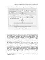
1.2. Range
Figure 1.5 shows a simplified pulsed radar block diagram. The time control
box generates the synchronization timing signals required throughout the sys-
tem. A modulated signal is generated and sent to the antenna by the modulator/
transmitter block. Switching the antenna between the transmitting and receiv-
ing modes is controlled by the duplexer. The duplexer allows one antenna to be
used to both transmit and receive. During transmission it directs the radar elec-
tromagnetic energy towards the antenna. Alternatively, on reception, it directs
the received radar echoes to the receiver. The receiver amplifies the radar
returns and prepares them for signal processing. Extraction of target informa-

tion is performed by the signal processor block. The target’s range, , is com-
puted by measuring the time delay, ; it takes a pulse to travel the two-way
path between the radar and the target. Since electromagnetic waves travel at
the speed of light, , then
R
∆
t
c
310
8
×
m
sec
⁄
=
Si
g
nal
p
rocessor
Time
Control
Transmitter
/
M odulator
Si
g
nal
p
rocessor

Receiver
R
Figure 1.5. A simplified pulsed radar block diagram.
Du
p
lexer
© 2000 by Chapman & Hall/CRC
(1.1)
where is in meters and is in seconds. The factor of is needed to
account for the two-way time delay.
In general, a pulsed radar transmits and receives a train of pulses, as illus-
trated by Fig. 1.6. The Inter Pulse Period (IPP) is , and the pulse width is .
The IPP is often referred to as the Pulse Repetition Interval (PRI). The inverse
of the PRI is the PRF, which is denoted by ,
(1.2)
During each PRI the radar radiates energy only for seconds and listens for
target returns for the rest of the PRI. The radar transmitting duty cycle (factor)
is defined as the ratio . The radar average transmitted power is
,
(1.3)
where denotes the radar peak transmitted power. The pulse energy is
.
The range corresponding to the two-way time delay is known as the radar
unambiguous range, . Consider the case shown in Fig. 1.7. Echo 1 repre-
sents the radar return from a target at range due to pulse 1. Echo
2 could be interpreted as the return from the same target due to pulse 2, or it
may be the return from a faraway target at range due to pulse 1 again. In
this case,
(1.4)
R

c
∆
t
2

=
R
∆
t
1
2

T
τ
f
r
f
r
1
PRI

1
T

==
time
time
transmitted
p
ulses

received
p
ulses
τ
IPP
p
ulse 1
∆
t
p
ulse 3
p
ulse 2
τ
p
ulse 1
echo
p
ulse 2
echo
p
ulse 3
echo
Figure 1.6. Train of transmitted and received pulses.
τ
d
t
d
t
τ

T
⁄
=
P
av
P
t
d
t
×
=
P
t
E
p
P
t
τ
P
av
TP
av
f
r
⁄
== =
T
R
u
R

1
c
∆
t
2
⁄
=
R
2
R
2
c
∆
t
2

=
or R
2
cT
∆
t
+
()
2

=
© 2000 by Chapman & Hall/CRC
Clearly, range ambiguity is associated with echo 2. Therefore, once a pulse is
transmitted the radar must wait a sufficient length of time so that returns from

targets at maximum range are back before the next pulse is emitted. It follows
that the maximum unambiguous range must correspond to half of the PRI,
(1.5)
MATLAB Function “pulse_train.m”
The MATLAB function “pulse_train.m” computes the duty cycle, average
transmitted power, pulse energy, and the pulse repetition frequency. It is given
in Listing 1.1 in Section 1.8; its syntax is as follows:
[dt pav ep prf ru] = pulse_train(tau,pri,p_peak)
where
Symbol Description Units Status
tau pulse width seconds input
pri PRI seconds input
p_peak peak power Watts input
dt duty cycle none output
pav average transmitted power Watts output
ep pulse energy Joules output
prf PRF Hz output
ru unambiguous range Km output
transmitted
p
ulses
received
p
ulses
τ
PRI
p
ulse 1
∆
t

p
ulse 2
echo1

echo 2
R
1
c
∆
t
2

=
R
u
R
2
∆
t
tim e or ran
g
e
time or ran
g
e
t
0=
t
1
f

r
⁄
=
Figure 1.7. Illustrating range ambiguity.
R
u
c
T
2

c
2
f
r

==
© 2000 by Chapman & Hall/CRC
Example 1.1: A certain airborne pulsed radar has peak power ,
and uses two PRFs, and . What are the required
pulse widths for each PRF so that the average transmitted power is constant
and is equal to ? Compute the pulse energy in each case.
Solution: Since is constant, then both PRFs have the same duty cycle.
More precisely,

The pulse repetition intervals are
It follows that
.

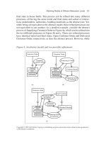
1.3. Range Resolution
Range resolution, denoted as , is a radar metric that describes its ability

to detect targets in close proximity to each other as distinct objects. Radar sys-
tems are normally designed to operate between a minimum range , and
maximum range . The distance between and is divided into
range bins (gates), each of width ,
(1.6)
Targets separated by at least will be completely resolved in range, as illus-
trated in Fig. 1.8. Targets within the same range bin can be resolved in cross
range (azimuth) utilizing signal processing techniques.
P
t
10
KW
=
f
r
1
10
KHz
=
f
r
2
30
KHz
=
1500
Watts
P
av
d

t
1500
10 10
3
×

0.15==
T
1
1
10 10
3
×

0.1
ms
==
T
2
1
30 10
3
×

0.0333
ms
==
τ
1
0.15

T
1
×
15
µ
s
==
τ
2
0.15
T
2
×
5
µ
s
==
E
p
1
P
t
τ
1
10 10
3
×
15 10
6–
××

0.15
Joules
== =
E
p
2
P
2
τ
2
10 10
3
×
510
6–
××
0.05
Joules
== =
∆
R
R
min
R
max
R
min
R
max
M

∆
R
M
R
max
R
min
–
∆
R

=
∆
R
© 2000 by Chapman & Hall/CRC