Fundementals of heat and mass transfer kotandaraman

This page
intentionally left
blank
Copyright © 2006, 1999, 1994, New Age International (P) Ltd., Publishers
Published by New Age International (P) Ltd., Publishers
All rights reserved.
No part of this ebook may be reproduced in any form, by photostat, microfilm,
xerography, or any other means, or incorporated into any information retrieval
system, electronic or mechanical, without the written permission of the publisher.
All inquiries should be emailed to
PUBLISHING FOR ONE WORLD
NEW AGE INTERNATIONAL (P) LIMITED, PUBLISHERS
4835/24, Ansari Road, Daryaganj, New Delhi - 110002
Visit us at www.newagepublishers.com
ISBN (13) : 978-81-224-2642-7
Professor Obert has observed in his famous treatise on Thermodynamics that concepts are
better understood by their repeated applications to real life situations. A firm conviction of
this principle has prompted the author to arrange the text material in each chapter in the
following order.
In the first section after enunciating the basic concepts and laws mathematical models
are developed leading to rate equations for heat transfer and determination of temperature
field, simple and direct numerical examples are included to illustrate the basic laws. More
stress is on the model development as compared to numerical problems.
A section titled “SOLVED PROBLEMS” comes next. In this section more involved
derivations and numerical problems of practical interest are solved. The investigation of the
effect of influencing parameters for the complete spectrum of values is attempted here. Problems
involving complex situations are shown solved in this section. Two important ideas are stressed
in this section. These are checking of dimensional homogeneity in the case of all equations

derived and the validation of numerical answers by cross checking. This concept of validation
in professional practice is a must in all design situations.
In the next section objective type questions are given. These are very useful for
understanding the basis and resolving misunderstandings.
In the final section a large number of graded exercise problems involving simple to
complex situations are included.
In the first of the 14 chapters the basic laws for the three modes of heat transfer are
introduced and the corresponding rate equations are developed. The use of electrical analogy
is introduced and applied to single and multimode heat transfer situations. The need for iterative
working is stressed in the solved problems.
The second chapter deals with one dimensional steady state conduction. Mathematical
models are developed by the three geometries namely Plate, Hollow Cylinder and Hollow Sphere.
Multilayer insulation is also discussed. The effect of variation of thermal conductivity on heat
transfer and temperature field is clearly brought out. Parallel flow systems are discussed.
Examples on variation of area along the heat flow direction are included. The use of electrical
analogy is included in all the worked examples. The importance of calculating the temperature
gradient is stressed in many of the problems.
In the third chapter models for conduction with heat generation are developed for three
geometric configurations namely plate, cylinder and sphere. The effect of volume to surface
area and the convection coefficient at the surface in maintaining lower material temperature
is illustrated. Hollow cylindrical shape with different boundary conditions is discussed.
Conduction with variable heat generation rate is also modelled.
Fins/extended surface or conduction-convection situation is discussed in the fourth
chapter. Models for heat transfer and temperature variation are developed for four different
PREFACE TO THE THIRD EDITION
boundary conditions. Optimisation of the shape of the fin of specified volume for maximum
heat flow is discussed. Circumferential fins and variable area fins are analysed. The use of
numerical method is illustrated. Error in measurement of temperature using thermometer is
well discussed. The possibility of measurement of thermal conductivity and convective heat
transfer coefficient using fins is illustrated.

Two dimensional steady state conduction is discussed in the fifth chapter. Exact analysis
is first developed for two types of boundary conditions. The use of numerical method is illustrated
by developing nodal equations. The concept and use of conduction shape factor is illustrated
for some practical situations.
One dimensional transient (unsteady) heat conduction is discussed in Chapter 6. Three
types of models arise in this case namely lumped heat capacity system, semi-infinite solid and
infinite solid. Lumped heat capacity model for which there are a number of industrial
applications is analysed in great detail and problems of practical interest are shown solved.
The condition under which semi-infinite solid model is applicable as compared to infinite solid
model is clearly explained. Three types of boundary conditions are analysed. Infinite solid
model for three geometric shapes is analysed next. The complexity of the analytical solution is
indicated. Solution using charts is illustrated in great detail. Real solids are of limited
dimensions and these models cannot be applied directly in these cases. In these cases product
solution is applicable. A number of problems of practical interest for these types of solids are
worked out in this section. In both cases a number of problems are solved using numerical
methods. Periodic heat flow problems are also discussed.
Concepts and mechanism of convection are discussed in the seventh chapter. After
discussing the boundary layer theory continuity, momentum and energy equations are derived.
Next the different methods of solving these equations are discussed. In addition to the exact
analysis approximate integral method, analogy method and dimensional analysis are also
discussed and their applicability is indicated. General correlations for convective heat transfer
coefficient in terms of dimensionless numbers are arrived at in this chapter.
In Chapter 8, in addition to the correlations derived in the previous chapter, empirical
correlations arrived at from experimental results are listed and applied to flow over surfaces
like flat plate, cylinder, sphere and banks of tubes. Both laminar and turbulent flows situation
are discussed.
Flow through ducts is discussed in Chapter 9. Empirical correlations for various situations
are listed. Flow developing region, fully developed flow conditions, constant wall temperature
and constant wall heat flux are some of the conditions analysed. Flow through non-circular
pipes and annular flow are also discussed in this chapter.

Natural convection is dealt with in Chapter 10. Various geometries including enclosed
space are discussed. The choice of the appropriate correlation is illustrated through a number
of problems. Combined natural and forced convection is also discussed.
Chapter 11 deals with phase change processes. Boiling, condensation, freezing and
melting are discussed. Basic equations are derived in the case of freezing and melting and
condensation. The applicable correlations in boiling are listed and their applicability is
illustrated through numerical examples.
Chapter 12 deals with heat exchangers, both recuperative and regenerative types. The
LMTD and NTU-effectiveness methods are discussed in detail and the applicability of these
methods is illustrated. Various types of heat exchangers are compared for optimising the size.
vi PREFACE
Thermal radiation is dealt with in Chapter 13. The convenience of the use of electrical
analogy for heat exchange among radiating surfaces is discussed in detail and is applied in
almost all the solved problems. Gas radiation and multi-body enclosures are also discussed.
Chapter 14 deals with basic ideas of mass transfer in both diffusion and convection
modes. A large number of problems with different fluid combinations are worked out in this
chapter.
A large number of short problems and fill in the blank type and true or false type
questions are provided to test the understanding of the basic principles.
Author
PREFACE vii
This page
intentionally left
blank
CONTENTS
Preface to the Third Edition v
1 AN OVERVIEW OF HEAT TRANSFER 1–25
1.0 Introduction 1
1.1 Heat Transfer 1
1.2 Modes of Heat Transfer 2

1.3 Combined Modes of Heat Transfer 8
1.4 Dimensions and Units 10
1.5 Closure 11
Solved Problems 11
Exercise Problems 22
2 STEADY STATE CONDUCTION 26–98
2.0 Conduction 26
2.1 The General Model for Conduction Study 26
2.2 Steady Conduction in One Direction (One Dimensional) 30
2.3 Conduction in Other Shapes 41
2.4 One Dimensional Steady State Heat Conduction with Variable Heat
Conductivity or Variable Area Along the Section 42
2.5 Critical Thickness of Insulation 48
2.6 Mean Area Concept 50
2.7 Parallel Flow 51
Solved Problems 53
Objective Questions 92
Exercise Problems 93
3 CONDUCTION WITH HEAT GENERATION 99–127
3.0 Introduction 99
3.1 Steady State One Dimensional Conduction in a Slab with Uniform Heat
Generation 99
3.2 Steady State Radial Heat Conduction in Cylinder with Uniform Heat Generation 103
3.3 Radial Conduction in Sphere with Uniform Heat Generation 107
3.4 Conclusion 109
Solved Problems 110
Objective Questions 125
Exercise Problems 125
VED
c-4\n-demo\tit ix

4 HEAT TRANSFER WITH EXTENDED SURFACES (FINS) 128–175
4.0 Introduction 128
4.1 Fin Model 129
4.2 Temperature Calculation 130
4.3 Heat Flow Calculation 134
4.4 Fin Performance 139
4.5 Circumferential Fins and Plate Fins of Varying Sections 142
4.6 Optimisation 145
4.7 Fin with Radiation Surroundings 146
4.8 Contact Resistance 146
4.9 Numerical Method 147
Solved Problems 148
Objective Questions 170
Exercise Problems 172
5 TWO DIMENSIONAL STEADY HEAT CONDUCTION 176–201
5.0 Introduction 176
5.1 Solution to Differential Equation 176
5.2 Graphical Method 182
5.3 Numerical Method 184
5.4 Electrical Analogy 187
5.5 In the Finite Difference Formulation 187
Solved Problems 188
Exercise Problems 199
6 TRANSIENT HEAT CONDUCTION 202–284
6.0 Introduction 202
6.1 A Wall Exposed to the Sun 202
6.2 Lumped Parameter Model 203
6.3 Semi Infinite Solid 207
6.4 Periodic Heat Conduction 213
6.5 Transient Heat Conduction in Large Slab of Limited Thickness, Long Cylinders

and Spheres 215
6.6. Product Solution 227
6.7 Numerical Method 230
6.8 Graphical Method 233
Solved Problems 234
Objective Questions 278
Exercise Problems 280
x CONTENTS
VED
c-4\n-demo\tit x
7 CONVECTION 285–333
7.0 Introduction 285
7.1 Mechanism of Convection 285
7.2 The Concept of Velocity Boundary Layer 287
7.3 Thermal Boundary Layer 289
7.4 Laminar and Turbulent Flow 291
7.5 Forced and Free Convection 292
7.6 Methods Used in Convection Studies 293
7.7 Energy Equation 299
7.8 Integral Method 302
7.9 Dimensional Analysis 303
7.10 Analogical Methods 306
7.11 Correlation of Experimental Results 307
Solved Problems 308
Objective Questions 331
Exercise Problems 332
8 CONVECTIVE HEAT TRANSFER—PRACTICAL CORRELATIONS
—FLOW OVER SURFACES 334–384
8.0 Introduction 334
8.1 Flow Over Flat Plates 334

8.2 Turbulent Flow 343
8.3 Flow Across Cylinders 348
8.4 Flow Across Spheres 356
8.5 Flow Over Bluff Bodies 359
8.6 Flow Across Bank of Tubes 360
Solved Problems 363
Objective Questions 380
Exercise Problems 381
9 FORCED CONVECTION 385–433
9.0 Internal Flow 385
9.1 Hydrodynamic Boundary Layer Development 386
9.2 Thermal Boundary Layer 387
9.3 Laminar Flow 388
9.4 Turbulent Flow 399
9.5 Liquid Metal Flow 402
9.6 Flow Through Non-circular Sections 404
9.7 The Variation of Temperature Along the Flow Direction 406
Solved Problems 408
Objective Questions 431
Exercise Problems 432
CONTENTS xi
VED
c-4\n-demo\tit xi
10 NATURAL CONVECTION 434–479
10.0 Introduction 434
10.1 Basic Nature of Flow Under Natural Convection Conditions 435
10.2 Methods of Analysis 437
10.3 Integral Method 439
10.4 Correlations from Experimental Results 442
10.5 A More Recent Set of Correlations 446

10.6 Constant Heat Flux Condition—Vertical Surfaces 447
10.7 Free Convection from Inclined Surfaces 451
10.8 Horizontal Cylinders 454
10.9 Other Geometries 455
10.10 Simplified Expressions for Air 456
10.11 Free Convection in Enclosed Spaces 458
10.12 Rotating Cylinders, Disks and Spheres 459
10.13 Combined Forced and Free Convection 460
Solved Problems 461
Objective Questions 477
Exercise Problems 477
11 PHASE CHANGE PROCESSES—BOILING, CONDENSATION
FREEZING AND MELTING 480–520
11.0 Introduction 480
11.1 Boiling or Evaporation 480
11.2 The correlations 483
11.3 Flow Boiling 485
11.4 Condensation 488
11.5 Freezing and Melting 494
Solved Problems 494
Objective Questions 516
Exercise Problems 518
12 HEAT EXCHANGERS 521–577
12.0 Introduction 521
12.1 Over All Heat Transfer Coefficient 521
12.2 Classification of Heat Exchangers 524
12.3 Mean Temperature Difference—Log Mean Temperature Difference 526
12.4 Regenerative Type 531
12.5 Determination of Area in Other Arrangements 531
12.6 Heat Exchanger Performance 535

12.7 Storage Type Heat Exchangers 547
12.8 Compact Heat Exchangers 550
xii CONTENTS
VED
c-4\n-demo\tit xii
Solved Problems 550
Objective Questions 572
Exercise Problems 574
13 THERMAL RADIATION 578–655
13.0 Introduction 578
13.1 Black Body 579
13.2 Intensity of Radiation 583
13.3 Real Surfaces 584
13.4 Radiation Properties of Gases—Absorbing, Transmitting and Emitting Medium 587
13.5 Heat Exchange by Radiation 595
13.6 Radiant Heat Exchange Between Black Surfaces 604
13.7 Heat Exchange by Radiation Between Gray Surfaces 606
13.8 Effect of Radiation on Measurement of Temperature by a Bare Thermometer 613
13.9 Multisurface Enclosure 614
13.10 Surfaces Separated by an Absorbing and Transmitting Medium 617
Solved Problems 618
Objective Questions 648
Exercise Problems 650
14 MASS TRANSFER 656–701
14.0 Introduction 656
14.1 Properties of Mixture 656
14.2 Diffusion Mass Transfer 657
14.3 Fick’s Law of Diffusion 657
14.4 Equimolal Counter Diffusion 659
14.5 Stationary Media with Specified Surface Concentration 660

14.6 Diffusion of One Component into a Stationary Component or
Unidirectional Diffusion 661
14.7 Unsteady Diffusion 661
14.8 Convective Mass Transfer 662
14.9 Similarity Between Heat and Mass Transfer 664
Solved Problems 664
Exercise Problems 680
Fill in the Blanks 682
State True or False 699
Short Questions 702
Appendix 707
References 712
CONTENTS xiii
This page
intentionally left
blank
VED
c-4\n-demo\tit xiii
Unit Conversion Constants
Quantity S.I. to English English to S.I.
Length 1 m = 3.2808 ft 1 ft = 0.3048 m
Area 1 m
2
= 10.7639 ft
2
1 ft
2
= 0.0929 m
2
Volume 1 m

3
= 35.3134 ft
3
1 ft
3
= 0.02832 m
3
Mass 1 kg = 2.20462 lb 1 lb = 0.4536 kg
Density 1 kg/m
3
= 0.06243 lb/ft
3
1 lb/ft
3
= 16.018 kg/m
3
Force 1 N = 0.2248 lb
f
1 lb
f
= 4.4482 N
Pressure 1 N/m
2
= 1.4504 × 10
–4
lb
f
/in
2
1 lb

f
/in
2
= 6894.8 N/m
2
Pressure 1 bar = 14.504 lb
f
/in
2
1 lb
f
/in
2
= 0.06895 bar
Energy 1 kJ = 0.94783 Btu 1 Btu = 1.0551 kJ
(heat, work) 1 kW hr = 1.341 hp hr 1 hp hr = 0.7457 kW hr
Power 1 W = 1.341 × 10
–3
hp 1 hp = 745.7 W
Heat flow 1 W = 3.4121 Btu/hr 1 Btu/hr = 0.29307 W
Specific heat 1 kJ/kg°C = 0.23884 Btu/lb°F 1 Btu/lb°F = 4.1869 kJ/kg°C
Surface tension 1 N/m = 0.068522 lb
f
/ft 1 lb
f
/ft = 14.5939 N/m
Thermal conductivity 1 W/m°C = 0.5778 Btu/hr ft°F 1 Btu/hrft°F = 1.7307 W/m°C
Convection coefficient 1 W/m
2
°C = 0.1761 Btu/hrft

2
°F 1 Btu/hr ft
2
°F = 5.6783 W/m
2
°C
Dynamic viscosity 1 kg/ms = 0.672 lb/fts 1 lb/fts = 1.4881 kg/ms
= 2419.2 lb/ft hr or Ns/m
2
Kinematic viscosity 1 m
2
/s = 10.7639 ft
2
/s 1 ft
2
/s = 0.092903 m
2
/s
Universal gas const. 8314.41 J/kg mol K
= 1545 ft lb
f
/mol R
= 1.986 B tu/lb mol R
Stefan Boltzmann const. 5.67 W/m
2
K
4
= 0.174 Btu/hr ft
2
R

4
VED
c-4\n-demo\tit xiv
Quantity S.I. to Metric Metric to S.I.
Force 1 N = 0.1019 kg
f
1 kg
f
= 9.81 N
Pressure 1 N/m
2
= 10.19 × 10
–6
kg
f
/cm
2
1 kg
r
/cm
2
= 98135 N/m
2
Pressure 1 bar = 1.0194 kg
f
/cm
2
1 kg
f
/cm

2
= 0.9814 bar
Energy 1 kJ = 0.2389 kcal 1 kcal = 4.186 kJ
(heat, work) 1 Nm (= 1 J) = 0.1019 kg
f
m 1 kg
f
m = 9.81 Nm (J)
Energy
(heat, work) 1 kWhr = 1.36 hp hr 1 hp hr = 0.736 kW hr
Power (metric) 1 W = 1.36 × 10
–3
hp 1 hp = 736 W
Heat flow 1 W = 0.86 kcal/hr 1 kcal/hr = 1.163 W
Specific heat 1 kJ/kg°C = 0.2389 kcal/kg°C 1 kcal/kg°C = 4.186 kJ/kg°C
Surface tension 1 N/m = 0.1019 kg
f
/m 1 kg
f
/m = 9.81 N/m
Thermal conductivity 1 W/m°C = 0.86 kcal/hrm°C 1 kcal/hrm°C = 1.163 W/m°C
Convection coefficient 1 W/m
2
°C = 0.86 kcal/hrm
2
°C 1 kcal/hrm
2
°C = 1.163 W/m
2
°C

Dynamic viscosity 1 kg/ms (Ns/m
2
) = 0.1 Poise 1 poise = 10 kg/ms (Ns/m
2
)
Kinematic viscosity 1 m
2
/s = 3600 m
2
/hr 1 m
2
/hr = 2.778 × 10
–4
m
2
/s
1 Stoke = cm
2
/s = 0.36 m
2
/hr = 10
–4
m
2
/s
Universal gas const. 8314.41 J/kg mol K = 847.54 m kg
f
/kg mol K
= 1.986 kcal/kg mol K
Gas constant in air (SI) = 287 J/kg K

Stefan Boltzmann const. 5.67 × 10
–8
W/m
2
K
4
= 4.876 × 10
–8
kcal/hr m
2
K
4
UNIT CONVERSION CONSTANTS xvi
VED
c-4\n-demo\demo1-1.pm5
1
AN OVERVIEW OF HEAT TRANSFER
1
1.0 INTRODUCTION
The present standard of living is made possible by the energy available in the form of heat
from various sources like fuels. The process by which this energy is converted for everyday use
is studied under thermodynamics, leaving out the rate at which the energy is transferred. In
all applications, the rate at which energy is transferred as heat, plays an important role. The
design of all equipments involving heat transfer require the estimate of the rate of heat transfer.
There is no need to list the various equipments where heat transfer rate influences their
operation.
The driving potential or the force which causes the transfer of energy as heat is the
difference in temperature between systems. Other such transport processes are the transfer of
momentum, mass and electrical energy. In addition to the temperature difference, physical
parameters like geometry, material properties like conductivity, flow parameters like flow

velocity also influence the rate of heat transfer.
The aim of this text is to introduce the various rate equations and methods of
determination of the rate of heat transfer across system boundaries under different situations.
1.1 HEAT TRANSFER
The study of heat transfer is directed to (i) the estimation of rate of flow of energy as heat
through the boundary of a system both under steady and transient conditions, and (ii) the
determination of temperature field under steady and transient conditions, which also will
provide the information about the gradient and time rate of change of temperature at various
locations and time. i.e. T (x, y, z, τ) and dT/dx, dT/dy, dT/dz, dT/dτ etc. These two are interrelated,
one being dependent on the other. However explicit solutions may be generally required for
one or the other.
The basic laws governing heat transfer and their application are as below:
1. First law of thermodynamics postulating the energy conservation principle: This
law provides the relation between the heat flow, energy stored and energy generated in a
given system. The relationship for a closed system is: The net heat flow across the system
bondary + heat generated inside the system = change in the internal energy, of the
system. This will also apply for an open system with slight modifications.
The change in internal energy in a given volume is equal to the product of volume
density and specific heat ρcV and dT where the group ρcV is called the heat capacity of the
system. The basic analysis in heat transfer always has to start with one of these relations.
Chapter 1
VED
c-4\n-demo\demo1-1.pm5
2 FUNDAMENTALS OF HEAT AND MASS TRANSFER
k
T
1
Q
T
2

x
1
L
x
2
Fig. 1.1. Physical model for
example 1.1
2. The second law of thermodynamics establishing the direction of energy transport
as heat. The law postulates that the flow of energy as heat through a system boundary will
always be in the direction of lower temperature or along the negative temperature gradient.
3. Newtons laws of motion used in the determination of fluid flow parameters.
4. Law of conservation of mass, used in the determination of flow parameters.
5. The rate equations as applicable to the particular mode of heat transfer.
1.2 MODES OF HEAT TRANSFER
1.2.1. Conduction: This is the mode of energy transfer as heat due to temperature
difference within a body or between bodies in thermal contact without the
involvement of mass flow and mixing. This is the mode of heat transfer through solid
barriers and is encountered extensively in heat transfer equipment design as well as in heating
and cooling of various materials as in the case of heat treatment. The rate equation in this
mode is based on Fourier’s law of heat conduction which states that the heat flow by
conduction in any direction is proportional to the temperature gradient and area
perpendicular to the flow direction and is in the direction of the negative gradient.
The proportionality constant obtained in the relation is known as thermal conductivity, k, of
the material. The mathematical formulation is given in equation 1.1.
Heat flow, Q = – kA dT/dx (1.1)
The units used in the text for various parameters are:
Q – W, (Watt), A – m
2
, dT – °C or K (as this is only temperature interval, °C and K can
be used without any difficulty). x – m, k – W/mK.

For simple shapes and one directional steady conditions with constant value of thermal
conductivity this law yields rate equations as below:
1. Conduction, Plane Wall (Fig. 1.1), the integration of the equation 1.1 for a plane
wall of thickness, L between the two surfaces at T
1
and T
2
under steady condition leads to
equation 1.2. The equation can be considered as the mathematical model for this problem.
Q =
TT
LkA
12
(/ )
−
(1.2)
Example 1.1: Determine the heat flow across a plane wall of 10 cm thickness with a constant
thermal conductivity of 8.5 W/mK when the surface temperatures are steady at 100°C and
30°C. The wall area is 3m
2
. Also find the temperature gradient in the flow direction.
Solution: Refer to Fig. 1.1 and equation 1.2:
T
1
= 100°C, T
2
= 30°C, L = 10 cm = 0.1 m,
k = 8.5 W/mK, A = 3 m
2
.

Therefore, heat flow, Q = (100 – 30) / (0.1/(8.5 × 3))
= 17850 W or 17.85 kW.
Referring to equation 1.1
Q = – kA dT/dx
17850 W = – 8.5 × 3 dT/dx.
Therefore dT/dx = – 17850/(8.5 × 3)
= – 700°C/m
VED
c-4\n-demo\demo1-1.pm5
AN OVERVIEW OF HEAT TRANSFER 3
Chapter 1
This is also equal to – (100 – 30)/0.1 = – 700°C/m, as the gradient is constant all through
the thickness.
Q
T
1
T
2
L/kA
I
V
1
V
2
R
(a) (b)
Fig. 1.2. Electrical analogy (a) conduction circuit (b) Electrical circuit.
The denominator in equation 1.2, namely L/kA can be considered as thermal resistance
for conduction. An electrical analogy is useful as a concept in solving conduction problems
and in general heat transfer problems.

1.2.2. Thermal Conductivity: It is the constant of proportionality in Fourier’s equation and
plays an important role in heat transfer. The unit in SI system for conductivity is W/mK. It is
a material property. Its value is higher for good electrical conductors and single crystals like
diamond. Next in order or alloys of metals and non metals. Liquids have conductivity less than
these materials. Gases have the least value for thermal conductivity.
In solids heat is conducted in two modes. 1. The flow of thermally activated electrons
and 2. Lattice waves generated by thermally induced atomic activity. In conductors the
predominant mode is by electron flow. In alloys it is equal between the two modes. In insulators,
the lattice wave mode is the main one. In liquids , conduction is by atomic or molecular diffusion.
In gases conduction is by diffusion of molecules from higher energy level to the lower level.
Thermal conductivity is formed to vary with temperature. In good conductors, thermal
conductivity decreases with temperature due to impedance to electron flow of higher
electron densities. In insulators, as temperature increases, thermal atomic activity also
increases and hence thermal conductivity increases with temperature. In the case of
gases, thermal conductivity increases with temperature due to increased random activity
of atoms and molecules. Thermal conductivity of some materials is given in table 1.1.
Table 1.1. Thermal conductivity of some materials at 293 K
Material Thermal conductivity, W/mK
Copper 386.0
Aluminium 204.2
Carbon Steel 1% C 43.3
Chrome Steel 20% Cr 22.5
Chrome Nickel Steel 12.8
Concrete 1.13
Glass 0.67
Water 0.60
Asbestos 0.11
Air 0.026
VED
c-4\n-demo\demo1-1.pm5

4 FUNDAMENTALS OF HEAT AND MASS TRANSFER
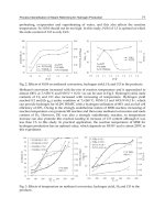
The variation of thermal conductivity of various materials with temperature is shown
in Fig. 1.3.
Silver(99.9%)
Aluminum(pure)
Magnesium(pure)
Lead
Mercury
Uo (dense)
2
Magnesite
Fireclay brick(burned 1330°C)
Carbon(amorphous)
Water
Hydrogen
Asbestos sheets
(40 laminations/m)
Engine oil
Copper(pure)
Air
CO
2
Solids
Liquids
Gases(at atm press)
100 0 100 200 300 400 500 600 700 800 900 1000
Temperature, °C
1000
100
10

1
0.1
0.01
0.001
Thermal conductivity k, (W/m °C)
Aluminum oxide
Iron(pure)
Fig. 1.3. Effect of temperature on thermal conductivity of materials.
1.2.3. Thermal Insulation: In many situations to conserve heat energy, equipments have to
be insulated. Thermal insulation materials should have a low thermal conductivity. This is
achieved in solids by trapping air or a gas in small cavities inside the material. It may also be
achieved by loose filling of solid particles. The insulating property depends on the material as
well as transport property of the gases filling the void spaces. There are essentially three types
of insulating materials:
1. Fibrous: Small diameter particles or filaments are loosely filled in the gap between
surfaces to be insulated. Mineral wool is one such material, for temperatures below 700°C.
Fibre glass insulation is used below 200°C. For higher temperatures refractory fibres like
Alumina (Al
2
O
3
) or silica (S
1
O
2
) are useful.
2. Cellular: These are available in the form of boards or formed parts. These contain
voids with air trapped in them. Examples are polyurethane and expanded polystyrene foams.
3. Granular: These are of small grains or flakes of inorganic materials and used in
preformed shapes or as powders.

The effective thermal conductivity of these materials is in the range of 0.02 to 0.04
W/mK.
VED
c-4\n-demo\demo1-1.pm5
AN OVERVIEW OF HEAT TRANSFER 5
Chapter 1
1.2.4. Contact Resistance: When two
different layers of conducting materials are
placed in thermal contact, a thermal
resistance develops at the interface. This
is termed as contact resistance. A
significant temperature drop develops at
the interface and this has to be taken into
account in heat transfer calculation. The
contact resistance depends on the surface
roughness to a great extent. The pressure
holding the two surfaces together also
influences the contact resistance. When the
surfaces are brought together the contact
is partial and air may be trapped between
the other points as shown in Fig. 1.4.
Some values of contact resistance for
different surfaces is given in table 1.2.
Table 1.2.
Surface type Roughness
µ
m Temp. Pressure atm R, m
2
°C/W × 10
4

Stainless Steel ground in air 2.54 20-200 3-25 2.64
Stainless Steel ground in air 1.14 20° 40-70 5.28
Aluminium ground air 2.54 150 12-25 0.88
Aluminium ground air 0.25 150 12-25 0.18.
1.2.5. Convection: This mode of heat transfer is met with in situations where energy is
transferred as heat to a flowing fluid at the surface over which the flow occurs. This mode is
basically conduction in a very thin fluid layer at the surface and then mixing caused by the
flow. The energy transfer is by combined molecular diffusion and bulk flow. The heat flow is
independent of the properties of the material of the surface and depends only on the fluid
properties. However the shape and nature of the surface will influence the flow and hence the
heat transfer. Convection is not a pure mode as conduction or radiation and hence involves
several parameters. If the flow is caused by external means like a fan or pump, then the
mode is known as forced convection. If the flow is due to the buoyant forces caused by
temperature difference in the fluid body, then the mode is known as free or natural convection.
In most applications heat is transferred from one fluid to another separated by a solid surface.
So heat is transferred from the hot fluid to the surface and then from the surface to the cold
fluid by convection. In the design process thus convection mode becomes the most important
one in the point of view of application. The rate equation is due to Newton who clubbed all the
parameters into a single one called convective heat transfer coefficient (h) as given in equation
1.3. The physical configuration is shown in Fig. 1.5. (a).
Fig. 1.4. Contact resistance temperature drop
T
2
T
c1
T
c2
T
1
T

DT
0
x
Insulated
Solid A
T
1
T
2
Solid B
Q Q
x
0
Insulated
Solid A
Solid B
Gap between solids
VED
c-4\n-demo\demo1-1.pm5
6 FUNDAMENTALS OF HEAT AND MASS TRANSFER
Heat flow, Q = hA (T
1
– T
2
) =
TT
hA
12
1/
−

(1.3)
where, Q → W.A → m
2
, T
1
, T
2
→ °C or K, ∴ h → W/m
2
K.
The quantity 1/hA is called convection resistance to heat flow. The equivalent circuit is
given in Fig. 1.5(b).
Surface
T
1
T
2
T>T
12
Fluid flow
Q
T
1
T
2
I/hA
Q
(a) (b)
Fig. 1.5. Electrical analogy for convection heat transfer
Example 1.2: Determine the heat transfer by convection over a surface of 0.5 m

2
area if the
surface is at 160°C and fluid is at 40°C. The value of convective heat transfer coefficient is 25
W/m
2
K. Also estimate the temperature gradient at the surface given k = 1 W/mK.
Solution: Refer to Fig. 1.5a and equation 1.3
Q = hA (T
1
– T
2
) = 25 × 0.5 × (160 – 40) W = 1500 W or 1.5 kW
The resistance = 1/hA = 1/25 × 0.5 = 0.08°C/W.
The fluid has a conductivity of 1 W/mK, then the temperature gradient at the surface
is
Q = – kA dT/dy
Therefore, dT/dy = – Q/kA
= – 1500/1.0 × 0.5 = – 3000°C/m.
The fluid temperature is often referred as T
∞
for indicating that it is the fluid temperature
well removed from the surface. The convective heat transfer coefficient is dependent on several
parameters and the determination of the value of this quantity is rather complex, and is
discussed in later chapters.
1.2.6. Radiation: Thermal radiation is part of the electromagnetic spectrum in the limited
wave length range of 0.1 to 10 µm and is emitted at all surfaces, irrespective of the temperature.
Such radiation incident on surfaces is absorbed and thus radiation heat transfer takes place
between surfaces at different temperatures. No medium is required for radiative transfer but
the surfaces should be in visual contact for direct radiation transfer. The rate equation is due
to Stefan-Boltzmann law which states that heat radiated is proportional to the fourth power

of the absolute temperature of the surface and heat transfer rate between surfaces is given in
equation 1.4. The situation is represented in Fig. 1.6 (a).
Q = F σ A (T
1
4
– T
2
4
) (1.4)
where, F—a factor depending on geometry and surface properties,
σ—Stefan Boltzmann constant 5.67 × 10
–8
W/m
2
K
4
(SI units)
A—m
2
, T
1
, T
2
→ K (only absolute unit of temperature to be used).
VED
c-4\n-demo\demo1-1.pm5
AN OVERVIEW OF HEAT TRANSFER 7
Chapter 1
This equation can also be rewritten as.
Q =

()
1/{ ( )( )}
12
121
2
2
2
TT
FAT T T T
−
++σ
(1.5)
where the denominator is referred to as radiation resistance (Fig. 1.6)
T
1
T
2
Q
1
F A (T + T )(T + T )s
11 2 1 2
22
A
2
T
2
(K)
Q
2
A

1
T
1
(K)
Q
1
T>T
12
(a) (b)
Fig. 1.6. Electrical analogy-radiation heat transfer.
Example 1.3: A surface is at 200°C and has an area of 2m
2
. It exchanges heat with another
surface B at 30°C by radiation. The value of factor due to the geometric location and emissivity
is 0.46. Determine the heat exchange. Also find the value of thermal resistance and equivalent
convection coefficient.
Solution: Refer to equation 1.4 and 1.5 and Fig. 1.6.
T
1
= 200°C = 200 + 273 = 473K, T
2
= 30°C = 30 + 273 = 303K.
(This conversion of temperature unit is very important)
σ = 5.67 × 10
–8
, A = 2m
2
, F = 0.46.
Therefore, Q = 0.46 × 5.67 × 10
–8

× 2[473
4
– 303
4
]
= 0.46 × 5.67 × 2 [(473/100)
4
– (303/100)
4
]
(This step is also useful for calculation and will be followed in all radiation problems-
taking 10
–8
inside the bracket).
Therefore, Q = 2171.4 W
Resistance can be found as
Q = ∆T/R, R = ∆T/Q = (200–30)/2171.4
Therefore, R = 0.07829°C/W or K/W
Resistance is also given by 1/h
r
A.
Therefore, h
r
= 6.3865 W/m
2
K
Check Q = h
r
A∆T = 6.3865 × 2 × (200–30) = 2171.4 W
The denominator in the resistance terms is also denoted as h

r
A. where h
r
= Fσ (T
1
+ T
2
)
(T
1
2
+ T
2
2
) and is often used due to convenience approximately h
r
= Fσ
TT
12
+
F
H
G
I
K
J
2
3
. The
determination of F is rather involved and values are available for simple configurations in the

form of charts and tables. For simple cases of black surface enclosed by the other surface F = 1
and for non black enclosed surfaces F = emissivity. (defined as ratio of heat radiated by a
surface to that of an ideal surface).
VED
c-4\n-demo\demo1-1.pm5
8 FUNDAMENTALS OF HEAT AND MASS TRANSFER
In this chapter only simple cases will be dealt with and the determination of F will be
taken up in the chapter on radiation. The concept of h
r
is convenient, though difficult to arrive
at if temperature is not specified. The value also increases rapidly with temperature.
1.3 COMBINED MODES OF HEAT TRANSFER
Previous sections treated each mode of heat transfer separately. But in practice all the three
modes of heat transfer can occur simultaneously. Additionally heat generation within the solid
may also be involved. Most of the time conduction and convection modes occur simultaneously
when heat from a hot fluid is transferred to a cold fluid through an intervening barrier. Consider
the following example. A wall receives heat by convection and radiation on one side. After
conduction to the next surface heat is transferred to the surroundings by convection and
radiation. This situation is shown in Fig. 1.7.
Q
R1
Q
cm1
L
T
¥1
T
¥2
T
2

T
1
k
Q
R2
12
Q
cm
T
¥1
1
hA
r1
1
hA
1
Q
L
kA
1
hA
r2
1
hA
2
T
¥
2
Fig. 1.7. Combined modes of heat transfer.
The heat flow is given by equation 1.6.

Q
A
TT
hh
L
kh h
rr
=
−
+
++
+
∞∞
12
11
12
12
(1.6)
where
h
r
1
and
h
r
2
are radiation coefficients and h
1
and h
2

are convection coefficients.
Example 1.4: A slab 0.2 m thick with thermal conductivity of 45 W/mK receives heat from a
furnace at 500 K both by convection and radiation. The convection coefficient has a value of
50 W/m
2
K. The surface temperature is 400 K on this side. The heat is transferred to surroundings
at
T
∞
2
both by convection and radiation. The convection coefficient on this side being 60 W/m
2
K.
Determine the surrounding temperature.
Assume F = 1 for radiation.
Solution: Refer Fig. 1.7. Consider 1 m
2
area. Steady state condition.
Heat received = σ (
TT
∞
−
1
4
1
4
) + h (T
∞1
– T
1

)
= 5.67
500
100
400
100
50 500 400
44
F
H
G
I
K
J
−
F
H
G
I
K
J
R
S
|
T
|
U
V
|
W

|
+−()
= 7092.2 W.