finance - turning finance into science - risk management and the black-scholes options pricing model

Turning Finance into Science:
Risk Management and the Black-
Scholes Options Pricing Model
Albert Kim
Mary Frauley
Writing for the Sciences
English ENG-LBE 09
Monday, May 1
st
2000
Recently, the people behind the famed Black- Scholes Options
Pricing Model received the Nobel Prize in Economics. Scientific
American delves into this formula that has its share of praise,
and criticism
A New Breed of $cience
In recent years, a new discipline called financial engineering has emerged
in order to attempt to understand finance using a scientific approach.
Mathematicians, physicists and traders work together in this discipline in order
to incorporate the use of advanced mathematics with everyday finance (Stix,
1998).
Although financial engineering deals with many aspects of finance, the
main application of this discipline is risk management within the stock market.
Regardless of what type of stock market transaction one performs, risk is
always present. However, it is the management of this risk that is studied by
these “financial engineers”. People need a fast and reliable way to calculate and
control the risk involved in all their stock trading.
This is where the Black- Scholes Option Pricing Model comes in. This
ideas behind this formula, created by Prof. Robert C. Merton, Prof. Myron S.
Scholes and the late Fisher Black, has been described by one economist as “the
most successful theory not only in finance but in all of economics.” (Stix, 1998)
Options

2
The functioning of the Black- Scholes Model is based on the use of stock
options. Stock options are a form of financial derivative (an item that is not a
stock in itself, but is an offshoot of one). It consists of a contract that gives
one the right, but not the obligation , to buy stocks later at a fixed price (known
as the exercise or strike price). The exercise price does not change, regardless
of all changes in the stock’s value. These options are purchased at a fee
known as the premium.
To illustrate, let’s say someone obtained the option to purchase 100
shares a year from now (a date known as the call date) for $100 each. If the
stock were to rise to $120 by the call date, it would be feasible for this person
to exercise his/her option, because the shares would still only cost you $100,
even though they are worth $120.
However, if the value of the stock were $80 at the call date, then it
would not be feasible to purchase these shares, because you would be paying
$100 for shares that are worth $80 each (a loss of $20 a share). Thus, this
person probably would not exercise his/her option, and would only lose the
premium he/she paid for the options a year ago.
Thus, stock options are a form of insurance policy. What makes stock
options so appealing is that the purchaser knows that the limit of his/her
3
losses can only be the premium price. However, there are no limits to his/her
gains, because the limit of the value of the stock is theoretically limitless
(Devlin, 1997).
The question is, what is the fair price for an option on a particular
stock? In other words, what is the option worth? When a stock has a call price
of $100 and a value of $120, the option is worth at least $20 ($120 - $100 =
$20). The value of the option clearly depends on the value of the stock. Thus,
if there were a formula that could tell you the fair price for an option while
taking into account all necessary factors, it would come of great use to the

financial world. This is what the Black- Scholes Options Pricing Model does.
The Math Behind It
Option pricing requires five inputs: the option’s exercise price, the time
to expiration, the price of the stock at the time of evaluation, current interest
rates and the volatility of the stock (Dammers, 1998). The only unreliable
factor is the volatility of the stock. This number can be estimated from
market data (Stix, 1998). The formula is as follows:
where the variable d is defined by:
4
According to this formula, the value of the option C, is given by the
difference between the expected share price (the first term) on the right- hand
side, and the expected cost (the second term) if the option is exercised. The
higher the current share price S, the higher the volatility of the share price
(Greek letter) sigma , the higher the interest rate r, the longer the time until the
call date t and the lower the strike price L, the higher the value of the option C
will be.
Limitations of the Model
As consistent as the model, there are limitations to the model. One
limitation is that it assumes that the options can only be exercised on the call
date. In other words, it cannot be exercised earlier. This model involves
“European- Style” options, rather than “American- Style” options. “American-
Style” options can be exercised anytime (Dammers, 1998). American options
are more flexible, thus more valuable. The model only takes European- style
options into account. Thus, the model underestimates the value of options.
Most options are not exercised until the call date anyways, but this law is not
written in stone.
5
Another limitation is that it assumes that the interest rate (determined
by the U.S. Government) is known and will remain more- or- less constant.
Many researchers have concluded that this is a safe assumption to make. But

there are times where the interest rate can change rapidly (Rubash, 1998), thus
putting the results of the model into question.
However, these limitations are considered insignificant, because they do
not affect the value of the option unless in extreme circumstances (such as a
sudden raise in interest rates or even a market crash).
The Birth of the Model
This formula did not create itself out of nowhere. Its roots lie deep in
the branches of mathematics known as probability and statistics. The
combination of these two domains of mathematics deals with the collection,
organization, and analysis of numerical data in order to assist decision-
making. In short, statistics let you “predict the future”, not with 100%
accuracy, but well enough so that you can make a wise decision as to your next
course of action (Devlin, 1997).
It all started when Charles Castelli wrote a book called “The Theory of
Options in Stocks and Shares” in 1877. Castelli’s book was the first to deal
with the use of options. However, this book lacked the theoretical basis
needed for actual application (Rubash, 1998).
6
Twenty- three years later, a graduate student by the name of Louis
Bachelier published his thesis paper “La Théorie de la Spéculation” (The
Theory of Speculation) at the Sorbonne, in Paris (Rubash, 1998). In this paper,
Bachelier dealt with the “structure of randomness” in the market. He
compared the behavior of buyers and sellers to the random movements of
particles suspended in fluids (NOVA Online, 2000). Remarkably, this paper
anticipated key insights developed later on by famed physicist Albert Einstein
and future theories in the field of probability.
He created the first complete mathematical model of options trading.
He believed the movements of stock prices were random and could never be
predicted, but risk could be managed (NOVA Online, 2000). He created a
formula that yielded an output that could help protect market investors from

excessive risk by means of pricing options. However, this formula contained
financially unrealistic assumptions, such as the existence of negative values
for stock prices and a zero interest rate (Stix, 1998). His paper was shelved
and went unnoticed for decades.
It wasn’t until 1955 that the idea of options pricing resurfaced, when a
professor at the Massachusetts Institute of Technology named Paul Samuelson
browsed through the Sorbonne library. He began developing a formula of his
own. Other mathematicians, such as Case Sprenkle and James Boness began
7
toying with Bachelier’s ideas as well (Royal Swedish Academy of Sciences,
1997). But all of their efforts went fruitless.
A Revolution
Then in 1968, a 31- year- old independent finance contractor named
Fisher Black and a 28- year- old assistant professor of finance at MIT named
Myron Scholes (Rubash, 1998) began their work on options pricing. They were
dissatisfied with all the formulas that had preceded them, because they were
overly complicated and made assumptions that didn’t make sense. They
wanted to find a formula that would calculate the fair price of an option at any
moment in time just by knowing the current price of the stock, but they
couldn’t see their way through the mass of equations they had inherited
(NOVA Online, 2000).
Then they decided to try something different. They decided to strip
previously derived formulas to their bare- boned state. They dropped
everything that represented something un- measurable (NOVA Online, 2000).
They were left with the vitals of calculating an option: the option’s exercise
price, the time to expiration, the price of the stock at the time of evaluation,
current interest rates and the volatility of the stock. But they were stuck with
one problem: one couldn’t measure volatility, or in other words, risk.
8
So they decided if they couldn’t measure the risk of an option, they

should make it less significant (NOVA Online, 2000). Their solution to this
problem was to become of the most celebrated discoveries of the 20
th
century.
The solution was rooted in the old gamblers’ practice of hedging. When one
makes a risky bet, one hedges his/her bet by also betting in the opposite
direction.
To illustrate, let’s say one were to bet that the favored Detroit Red Wings
would beat the Colorado Avalanche in a 2
nd
round playoff series. If one
already bet $50 on the Red Wings, one would hedge that bet by betting $45 on
the Avalanche. Although Detroit is favored, by hedging this bet with a slightly
smaller bet on Colorado, we are protecting ourselves in the event of a
Coloradoan upset. We minimize risk at the cost of lowering our possible
winnings. However, since Detroit is favored, the chances of winning $5 are
substantial.
A more business- oriented example would be as such: Let’s say a British
company is expecting to make several large payments in US dollars in a few
months. They can hedge against a huge drop in the Sterling Pound (thus
making it more expensive to buy US dollars) by purchasing options for US
dollars on a foreign currencies market. Effective risk management requires
that such options be correctly priced (Royal Swedish Academy of Sciences,
1997).
9
Fig 1: Hedging Cash Flows [Stix, G. (1998, May). A Calculus of Risk. Scientific American ,
p.94.]
To hedge against risks in changes in share price, the investor can buy
two options for every share he or she owns; the profit will then counter the
loss. Hedging creates a risk free portfolio (Stix, 1998). As the share price

changes over time, the investor must alter the composition of the portfolio,
the ratio of number of shares to the number of options, to ensure that the
holdings remain without risk (Stix, 1998).
They made up a theoretical portfolio of stocks and options. Whenever
either fluctuated up or down, they tried to hedge against the movement by
10
making another move in the opposite direction. Their aim was to keep the
overall value of the portfolio in perfect balance. In other words, they tried to
minimize risk.
They discovered that they could indeed reduce risk by creating a balance
in which all movements in the markets cancelled each other out. Black and
Scholes had found a theoretical way to neutralize risk (NOVA Online, 2000).
With risk now virtually eliminated from their equation, they had a
mathematical formula that could give them the price of any option. This was a
marvelous achievement.
There was a practical problem with their formula. It assumed that
markets were always in equilibrium, that supply equals demand (NOVA Online,
2000). They needed a way to instantly rebalance a portfolio of stocks and
options to keep countering all their movements.
A Harvard graduate by the name of Robert Merton solved this problem
by introducing the notion of continuous time. This idea is rooted in rocket
science. A Japanese mathematician by the name of Kiyosi Ito theorized that
when you plot the trajectory of a rocket, knowing where the rocket was
second- by- second was not enough. You needed to know where the rocket
was continuously. So he broke time down into infinitely small increments,
11
thus smoothening the graphing of its path out until it became a continuum so
that the trajectory could be constantly updated (NOVA Online, 2000). Merton
applied this idea to the Black- Scholes model so that the value of an option
could be constantly recalculated and risk eliminated continually (NOVA Online,

2000).
In 1997, Robert Merton and Myron Scholes were awarded the Nobel
prize in economic sciences for their efforts. Their colleague Fisher Black had
unfortunately passed away in 1994. (Royal Swedish Academy of Sciences,
1997).
The History of the Model
In 1973, the Chicago Options Exchange was launched, one month before
the Black- Scholes model was published (Stix, 1998). When these three men
had published their paper in 1973 in the Journal of Political Economy, traders,
academics and economists marveled at its overwhelming power, despite the
simple nature of its use.
Traders began using their ideas immediately. Texas Instruments had
incorporated their formula into their latest calculator, announcing their
feature in the Wall Street Journal (Devlin, 1997). The options market exploded
soon after.
12
So overwhelming was the sudden mass use of the Black- Scholes Model,
that when the stock market crashed in 1978, the influential business magazine
Forbes put the blame squarely onto that one formula (Devlin, 1997).
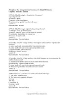
According to Capital Market Risk Advisors, about 20 percent of the
$23.77 billion (US) in derivatives losses in the last decade are due to problems
related to modeling (Stix, 1998). In 1997, however, model risk comprised
nearly 40 percent of the $2.65 billion (US) in money lost.
Fig 2: Derivatives Losses [Stix, G. (1998, May). A Calculus of Risk. Scientific American , p.
95.]
At a conference in February 1998, an industry trade magazine called
Derivatives Strategy sponsored a discussion group called “First Kill All the
Models”. (Stix, 1998) This group reflects the recent backlash against financial
13
models. Many figures in the financial industry question whether models can

match traders’ skill and gut intuition about market dynamics (Royal Swedish
Academy of Sciences, 1997).
Derivatives make the news because, like an airplane crash, their losses
can dramatic and chaotic. Enormous losses by Proctor & Gamble and Gibson
Greetings and the bankruptcies of Barings Bank and Orange County, California
have been attributed to the use of models (Stix, 1998).
Fig 3: Derivatives Debacles [Stix, G. (1998, May). A Calculus of Risk. Scientific American ,
pp. 91.]
14
However, Scholes says that it was not so much the formula itself that
caused these losses, rather its misuse by market traders. Every statistician
and mathematician knows you cannot predict the future with 100% accuracy.
Laws as rigid as the laws of physics do not govern the market. Peter Fisher, a
New York economist says: “Math doesn’t drive financial markets, people drive
financial markets, and people are not predictable. We do not yet have a
universal theory of human behavior or human motivation.” (NOVA Online,
2000)
It was not the model by itself that caused these losses, but the blind
faith that market traders put into it. They all jumped at the prospect of
making money without risk. However, this formula cannot eliminate risk, it
can only minimize it. Like many mathematical models, it relies on imputs and
assumes a functioning market. It is a powerful way to manage risk, but it’s not
a crystal ball. Scholes says this equation should be used as a tool for making
decisions, not a platform from which all decisions should be made (NOVA
Online, 2000).
Fisher says: “If a random bolt of lightning hits you when you’re
standing in the middle of the field, that feels like a random event. But if your
business is to stand in random fields during lightning storms, then you should
anticipate, perhaps a little more robustly, the risks you’re taking on.” (NOVA
15

Online, 2000) This formula is a method to calculate these risks, not a risk
neutralizer.
“There is a danger of accepting models without carefully questioning
them,” says Joseph A. Langsam, a former mathematician who develops and
tests models for fixed- income securities at Morgan Stanley (Stix, 1998). Thus,
the Black- Scholes is not the culprit for all derivative losses, but traders’ blind
faith in them.
Numbers vs. Instinct
Many traders still use the ideas behind the Black- Scholes Options
Pricing Model, if not the model itself. The fundamental ideas behind the
equation forever changed the stock market. Today, traders use many
principles of the Black- Scholes Model as guides through the treacherous
waters of the stock market. For this, Scholes and Fisher became Nobel
laureates. But the lessons of putting all of one’s eggs in the same “Black-
Scholes Model” basket have been learned. One cannot blindly put all his/her
faith into the model and expect guaranteed financial success. Judgment is still
required.
Samuelson says: “There is a tempting and fatal fascination in
mathematics. Albert Einstein warned against it. He said elegance is for tailors,
16
don’t believe in something because it’s a beautiful formula. There will always
be room for judgment.” (NOVA Online, 2000)
17
References:
Dammers, Jerry. (1998). “Option Pricing: The Concept & the Black- Scholes
Method” Valuemetrics, Inc. [Online] 4.9 (2000): Available URL:
/>Devlin, Keith. (November 1997). “A Nobel Formula.” Mathematical
Association of America. [Online] 4.9 (2000): Available URL:
/>Hull, J.C. (1997). Options, Futures, and other Derivatives. New York:
Prentice Hall.

NOVA Online. (Feb 8 2000) “Trillion Dollar Bet”. Public Broadcasting
Syndicate Homepage. [Online] 4.9 (2000): Available URL:
/>Ross, Sheldon M. (1999). An Introduction to Mathematical Finance: Options
and other Topics. Cambridge, MA: Cambridge University Press.
Royal Swedish Academy of Sciences. (1997) “Additional background
material on the Bank of Sweden Prize in Economic Sciences in Memory of Alfred
18
Nobel 1997.” The Official Website of the Nobel Foundation [Online] 4.9 (2000):
Available URL: 97/ecoback97.html
Rubash, Kevin. (1998) “A Study of Option Pricing Models” Bradley
University. [Online] 4.9 (2000): Available URL: />7Earr/bsm /m odel.html
Stix, G. (1998, May). A Calculus of Risk. Scientific American , pp. 90- 98.
19