atomic force microscopy, biomedical methods and applications

Methods in Molecular Biology
TM
Methods in Molecular Biology
TM
Edited by
Pier Carlo Braga
Davide Ricci
Atomic Force
Microscopy
VOLUME 242
Biomedical Methods and
Applications
Edited by
Pier Carlo Braga
Davide Ricci
Atomic Force
Microscopy
Biomedical Methods and
Applications
How AFM Works 3
3
1
How the Atomic Force Microscope Works
Davide Ricci and Pier Carlo Braga
1. Introduction
Microscopes have always been one of the essential instruments for research
in the biomedical field. Radiation-based microscopes (such as the light micro-
scope and the electron microscope) have become trustworthy companions in
the laboratory and have contributed greatly to our scientific knowledge. How-
ever, although digital techniques in recent years have still enhanced their per-
formance, the limits of their inherent capabilities have been progressively

reached.
The advent of scanning probe microscopes and especially of the atomic force
microscope (AFM; ref. 1) has opened new perspectives in the investigation of
biomedical specimens and induces to look again with rejuvenated excitement
at what we can learn by “looking” at our samples. Novices are at first mesmer-
ized by two features: the name of the instrument and the colorful 3D computer
visualization of surfaces. One later learns that quite often it is not possible to
obtain the “atomic” resolution that one hoped to achieve (2–4) but that never-
theless images do contain details not observable with any other instrument.
The tri-dimensional mapping of the surface gains scientific relevance when
one realizes that it is not just fancy surface reconstruction but that true topo-
graphic data with vertical resolution down to the subnanometer range is readily
available. Moreover, when simplified sample preparation and the possibility of
investigating specimens in liquid environment become apparent, one becomes
convinced that he or she must find a way to apply AFM to his or her own
research.
2. Performance Range of AFM
AFM images show significant information about surface features with
unprecedented clarity. The AFM can examine any sufficiently rigid surface
From:
Methods in Molecular Biology, vol. 242: Atomic Force Microscopy: Biomedical Methods and Applications
Edited by: P. C. Braga and D. Ricci © Humana Press Inc., Totowa, NJ
4 Ricci and Braga
either in air or with the specimen immersed in a liquid. Recently developed
instruments can allow temperature control of the sample, can be equipped with
a closed chamber for environmental control, and can be mounted on an inverted
microscope for simultaneous imaging through advanced optical techniques.
The field of view can vary from the atomic and molecular scale up to sizes
larger than 125 µm so that data can be compared with other information
obtained with lower resolution techniques. The AFM can also examine rough

surfaces because its vertical range can be up to 8–10 µm. Large samples can be
fitted directly in the microscope without cutting. With stand-alone instruments,
any area on flat or nearly flat specimens can be investigated. In addition to its
superior resolution with respect to optical microscopes, the AFM has these key
advantages with respect to electron microscopes. Compared with the scanning
electron microscope (SEM), the AFM provides superior topographic contrast,
in addition to direct measurements of surface features providing quantitative
height information.
Because the sample need not be electrically conductive, no metallic coating
of the sample is required. Hence, no dehydration of the sample is necessary as
with SEM, and samples may be imaged in their hydrated state. This eliminates
the shrinkage of biofilm associated with imaging using SEM, yielding a non-
destructive technique. The resolution of AFM is higher than that of environ-
mental SEM, where hydrated images can also be obtained and extracellular
polymeric substances may not be imaged.
Compared with transmission electron microscopes, 3D AFM images are
obtained without expensive sample preparation and yield far more complete
information than the 2D profiles available from cross-sectioned samples.
In the following subheadings we will give a brief outline of how the AFM
works followed by a description of the parts that can be added to the basic
instrument. Our overview makes no pretense to completeness but aims at sim-
plicity. For a more thorough description of the physical principles involved in
the operation of these instruments, we refer you to the specialized literature.
3. The Microscope
In Fig. 1, a schematic diagram of an AFM is shown (1,5). In principle, AFM
can bring to mind the record player, but it incorporates a number of refine-
ments that enable it to achieve atomic-scale resolution, such as very sharp tips,
flexible cantilevers, a sensitive deflection sensor, and high-resolution tip–
sample positioning.
3.1. The Tip and Cantilever

The tip, which is mounted at the end of a small cantilever, is the heart of the
instrument because it is brought in closest contact with the sample and gives
How AFM Works 5
rise to the image though its force interactions with the surface. When the first
AFM was made, a very small diamond fragment was carefully glued to one
end of a tiny piece of gold foil. Today, the tip–cantilever assembly typically is
fabricated from silicon or silicon nitride and, using technology similar to that
applied to integrated circuit fabrication, allows a good uniformity of character-
istics and reproducibility of results (6,7). The essential parameters are the
sharpness of the apex, measured by the radius of curvature, and the aspect ratio
of the whole tip (Fig. 2).
Although it would seem that sharper tips should yield more detailed images,
this may not occur with all samples: in fact, quite often, so-called “atomic
resolution” on crystals is obtained best with standard silicon nitride tips. In
general, one can choose among one of three types of tip. The standard tip is
usually a 3-µm tall pyramid with approx 30-nm end radius. The electron-beam-
deposited tip or “super tip” improves on this with an electron-beam–induced
deposit of material at the apex of the tip, offering a higher aspect ratio and end
radius than the normal tip, albeit with the drawback of fragility. Finally, tips
made from silicon (either polysilicon or single crystal) through improved
Fig. 1. Schematic diagram of a scanned-sample AFM. In the case of scanned probe,
it is the tip that is scanned instead of the sample. 1, Laser diode; 2, cantilever; 3,
mirror; 4, position-sensitive photodetector; 5, electronics; and 6, scanner with sample.
6 Ricci and Braga
microlithographic techniques have a higher aspect ratio and small apex radius
of curvature, maintaining reproducibility and durability (8).
The cantilever carrying the tip is attached to a small glass “chip” that allows
easy handling and positioning in the instrument. There are essentially two
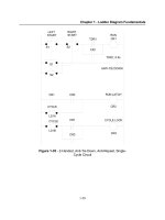
designs for cantilevers, the “V” shaped and the single-arm kind (Fig. 3), which
have different torsional properties. The length, width, and thickness of the

beam(s) determine the mechanical properties of the cantilever and have to be
chosen depending on mode of operation needed and on the sample to be inves-
tigated. Cantilevers are essentially classified by their force (or spring) constant
and resonance frequency: soft and low-resonance frequency cantilevers are
more suitable for imaging in contact and resonance mode in liquid, whereas
stiff and high-resonance frequency cantilevers are more appropriate for reso-
nance mode in air (9).
3.2. Deflection Sensor
AFMs can generally measure the vertical deflection of the cantilever with
picometer resolution. To achieve this, most AFMs today use the optical lever
or beam-bounce method, a device that achieves resolution comparable to an
interferometer while remaining inexpensive and easy to use.
In this system, a laser beam is reflected from the backside of the cantilever
(often coated by a thin metal layer to make a mirror) onto a position-sensitive
Fig. 2. The essential parameters in a tip are the radius of curvature (r) and the aspect
ratio (ratio of h to w).
How AFM Works 7
photodetector consisting of two side-by-side photodiodes. In this arrangement,
a small deflection of the cantilever will tilt the reflected beam and change the
position of beam on the photodetector. The difference between the two photo-
diode signals indicates the position of the laser spot on the detector and thus
the angular deflection of the cantilever.
Because the distance between cantilever and detector is generally three
orders of magnitude greater than the length of the cantilever (millimeters com-
pared to micrometers), the optical lever greatly magnifies motions of the tip
giving rise to an extremely high sensitivity.
3.3. Image Formation
Images are formed by recording the effects of the interaction forces between
tip and surface as the cantilever is scanned over the sample. The scanner and
the electronic feedback circuit, together with sample, cantilever, and optical

lever form a feedback loop set up for the purpose. The presence of a feedback
loop is a key difference between AFM and older stylus-based instruments so
that AFM not only measures the force on the sample but also controls it, allow-
ing acquisition of images at very low tip-to-sample forces (5,10).
The scanner is an extremely accurate positioning stage used to move the tip
over the sample (or the sample under the tip) to form an image, and generally
in modern instruments is made from a piezoelectric tube. The AFM electronics
drives the scanner across the first line of the scan and back. It then steps in the
Fig. 3. Triangular (A) and single-beam (B) cantilevers. The mechanical properties,
such as the force constant and resonant frequency, depend on the values of width (W),
length (L), and thickness (T).
8 Ricci and Braga
perpendicular direction to the second scan line, moves across it and back, then
to the third line, and so forth (Fig. 4).
As the probe is scanned over the surface, a topographic image is obtained
storing the vertical control signals sent by the feedback circuit to the scanner
moving it up and down to follow the surface morphology while keeping the
interaction forces constant. The image data are sampled digitally at equally
spaced intervals, generally from 64 up to 2048 points per line. The number of
lines is usually chosen to be equal to the number of data points per line, obtain-
ing at the end a square grid of data points each corresponding to the relative x,
y, and z coordinates in space of the sample surface (11).
Usually during scanning data are represented by gray scale images, in which
the brightness of points can range from black to white across 256 levels corre-
sponding to the information acquired by the microscope (that can be height,
force, phase, and so on).
4. A Variety of Instruments and Options
The first instruments introduced on the market had all very similar features
and range of applications: they had scanners with small range, limited optical
access, and could accommodate only small samples. Essentially they where

built to make very high-resolution imaging on flat samples in a dry environ-
ment. As the possibilities of AFM were developed, a wider range of instru-
ments, optimized for specific applications, have been developed. We can now
find instruments that are specifically designed for large samples, such as sili-
con wafers, that have metrological capabilities, utilize scanner close loop
operation, are optimized for liquid and electrochemistry operation, and can be
Fig. 4. Raster scan for image acquisition. The AFM electronics drive the scanner
across the first line of the scan and back. The scanner then steps in the perpendicular
direction to the second scan line, moves across it and back, then to the third line, and
so forth.
How AFM Works 9
mounted on an inverted microscope for biological investigations. Usually, one
single instrument can have different options to extend its capabilities, but to
date it is not possible to have an instrument that covers all possible applica-
tions with maximum performance. For this reason, it is necessary to have
clearly in mind what will be the main features that are desired in an instrument
before its purchase, understanding at the same time that a loss of performance
in other aspects may be possible.
One can distinguish between two main classes: scanned-sample and
scanned-tip microscopes. We give a brief description of the advantages of one
system with respect to the other.
4.1. Scanned Sample
This scanned-sample AFM is the first design in which the sample is attached
to the scanner and moved under the tip. Depending on how the cantilever
holder, laser, and photodetector are assembled, it can easily accommodate an
overhead microscope provided that long focal length objectives are used. A
clear view of where the tip is landing is usually possible, speeding up the time
it takes to get a meaningful image of the sample.
Scanners with wide x,y, and z range are usually available and closed loop
control feedback is more easily implemented in this scheme and often a lower

mechanical noise level can be obtained allowing higher ultimate resolution.
There are quite a few drawbacks. First of all, the size and weight of the
sample has to be limited because it is sitting on the scanner and may change its
behavior. For the same reason, operation in liquid is impaired because liquid
cells tend to be small and difficult to seal, and liquid flow or temperature con-
trol are more complicated to implement. Notwithstanding these difficulties,
excellent results can be obtained on typical biomedical science specimens by
ingeniously adapting them to the instruments characteristics.
4.2. Scanned Tip
In the scanned-tip method of operation, the sample stays still and it is the
cantilever, attached to the scanner, which is moved across the surface. Although
for scanning tunneling microscopes this was one of the first solutions applied,
to build a scanned tip AFM requires overcoming some difficulties, essentially
related to adapting the beam bounce detection scheme to a moving cantilever.
For this reason, it has been only recently that models made according to this
design have been marketed, after appropriate technology was developed. The
first examples were the so-called “stand-alone” systems, usually an AFM rest-
ing on three legs and able to scan the surface of any object under its probe.
Later, specialized instruments were developed, capable of being coupled or
even integrated into inverted optical microscopes for biological applications.
10 Ricci and Braga
With respect to the scanned-sample models, scanned-tip instruments can be
more easily equipped with temperature-controlled stages, open or closed liq-
uid cells, liquid flow systems, electrochemistry cells, and controlled atmo-
sphere chambers. Concerning limitations, one could say that what is gained on
one side is lost on the other. For example, often the overall noise level is higher,
limiting ultimate resolution. Large scan areas are more difficult to scan because
tracking systems have to be used to keep the laser spot on the back of the
cantilever. A top view of samples is obstructed by the scanner assembly: spe-
cial hollow tubes have been developed recently, but even so on-axis micro-

scopes, which are useful on nontransparent samples, will still have limited
resolution and lateral field of view.
5. Loading a Sample in the Microscope
5.1. Imaging Dry Samples
Samples to be imaged in atmospheric environment are often simply glued to
a sample holder, usually a metal disk. The disk is then inserted in the AFM,
where it is held firmly by a small magnet. An essential point is that the sample
has to be firmly adherent to the sample holder; otherwise, very poor imaging
will be achieved. For this reason, one has to be careful in the choice of the glue
or sticky tape: slow drying glue or thick sticky tape should be avoided. A draw-
back is that after use in the AFM, the sample is difficult to take off without
damage.
Some systems, usually scanned-tip, can accept samples directly, securing
them with a metal clip or springs. This method allows sample recovery without
damage for further use in other experiments, but it can be less stable and needs
special care for high-resolution work.
Sometimes, because of the ease of use of the AFM, one forgets to be careful
while handling the sample and either fingerprints or dust from a dirty environ-
ment contaminates the sample. It is best to keep a reserved area of the labora-
tory free from contaminants for the operations of sample and cantilever
mounting.
5.2. Imaging in Liquid
One of the main reasons for the success of AFM in biomedical investiga-
tions is its ability to scan samples in physiological condition, that is, immersed
in liquid solutions (12,13). Just to make an example, scanned-tip systems can
often be directly used to image cells into a standard Petri dish. Each manufac-
turer has its own design of liquid cells, sometimes different ones depending on
the application, and users may decide to make their own to fit specific needs. A
few additional things that have to be taken care of when imaging in liquid are
How AFM Works 11

the temperature of the solution (eventually added during imaging; ref. 14) and
maintenance of the liquid cell and cantilever holder assembly. Because the
cantilever is extremely sensitive to temperature changes, it is important to let
the system equilibrate before taking images. For example, in the case of con-
tact mode imaging with silicon nitride cantilevers and tips, a large change in
time of the signal on the photodetector corresponding to cantilever deflection
can be observed in the presence of a temperature change (15). If temperature is
not stable prior to approach of the tip to the sample and one starts taking images,
after some time the applied force could be quite different than at the beginning
of the imaging session.
Once finished using the microscope for imaging in liquid, it is essential to
immediately clean thoroughly all parts that have been in contact with the solu-
tion to avoid contamination of future experiments. Usually, it should be pos-
sible to disassemble and sonicate all vital parts of the liquid cell and the
cantilever holder.
6. Future Developments
The AFM is part of a family of scanning probe microscopes that has a great
growth potential. It is a fact that the majority of novel applications and tech-
niques developed in scanning probe microscopes in the last years are related to
the life sciences. There is still much room for technical improvement: electron-
ics, scanners, and tips are constantly improving. Scan speed limitations, sample
accessibility, and ease of use have been addressed and can be still improved. As
more and more biomedical researchers will be involved in the use of AFM, with
their experience they will be able contribute in developing an instrument less
related to the physical science (its origin) and more tailored to our specific needs.
References
1. Binnig, G., Quate, C. F., and Gerber, Ch. (1986) Atomic force microscope. Phys.
Rev. Lett. 56, 930–933.
2. Binnig, G., Gerber, C., Stoll, E., Albrecht, T. R., and Quate, C. F. (1987) Atomic
resolution with the atomic force microscope. Europhys. Lett. 3, 1281–1286.

3. Hug, H. J., Lantz, M. A., Abdurixit, A., et al. (2001) Subatomic features in atomic
force microscopy images. Science 291, 2509.
4. Jarvis, M. R., Perez, R., and Payne, M. C. (2001) Can atomic force microscopy
achieve atomic resolution in contact mode? Phys. Rev. Lett. 86, 1287–1290.
5. Alexander, S., Hellemans, L., Marti, O., et al. (1989) An atomic-resolution atomic-
force microscope implemented using an optical lever. J. Appl. Phys. 65, 164–167.
6. Albrecht, T. R., Akamine, S., Carver, T.E., and Quate, C. F. (1990) Microfabrication of
cantilever styli for the atomic force microscope. J. Vac. Sci. Technol. A 8, 3386–3396.
7. Tortonese, M. (1997). Cantilevers and tips for atomic force microscopy. IEEE
Engl. Med. Biol. Mag. 16, 28–33.
12 Ricci and Braga
8. Sheng, S., Czajkowsky, D. M., and Shao, Z. (1999) AFM tips: How sharp are
they? J. Microsc. 196, 1–5.
9. Cleveland, J. P., Manne, S., Bocek, D., and Hansma, P. K. (1993) A non-destruc-
tive method for determining the spring constant of cantilevers for scanning force
microscopy. Rev. Sci. Instrum. 64, 403–405.
10. Meyer, G. and Amer, N. M. (1988) Novel approach to atomic force microscopy.
Appl. Plrys. Lett. 53, 1045–1047.
11. Baselt, D. R., Clark, S. M., Youngquist, M. G., Spence, C. F., and Baldeschwieler,
J. D. (1993) Digital signal control of scanned probe microscopes. Rev. Sci.
Instrum. 64, 1874–1882.
12. Wade, T., Garst, J. F., and Stickney, J. L. (1999). A simple modification of a
commercial atomic force microscopy liquid cell for in situ imaging in organic,
reactive or air sensitive environments. Rev. Sci. Instr. 70, 121–124.
13. Lehenkari, P. P., Charras, G. T., Nykanen, A., and Horton, M. A. (2000) Adapting
atomic force microscopy for cell biology. Ultramicroscopy 82, 289–295.
14. Workman, R. K. and Manne, S. (2000) Variable temperature fluid stage for atomic
force microscopy. Rev. Sci. Instrum. 71, 431–436.
15. Radmacher, M., Cleveland, J. P., and Hansma, P. K. (1995) Improvement of ther-
mally induced bending of cantilevers used for atomic force microscopy. Scanning

17, 117–121.
Imaging Methods in AFM 13
13
2
Imaging Methods in Atomic Force Microscopy
Davide Ricci and Pier Carlo Braga
1. Introduction
One can easily distinguish between two general modes of operation of the
atomic force microscope (AFM) depending on absence or presence in the
instrumentation of an additional device that forces the cantilever to oscillate in
the proximity of its resonant frequency. The first case is usually called static
mode, or DC mode, because it records the static deflection of the cantilever,
whereas the second takes a variety of names (some patented) among which we
may point out the resonant or AC mode. In this case, the feedback loop will try
to keep at a set value not the deflection but the amplitude of the oscillation of
the cantilever while scanning the surface. To do this, additional electronics are
necessary in the detection circuit, such as a lock-in or a phase-locked loop
amplifier, and also in the cantilever holder to induce the oscillatory excitation.
From a physical point of view, one can make a distinction between the two
modes depending on the sign of the forces involved in the interaction between
tip and sample, that is, by whether the forces there are attractive or repulsive
(1). In Fig. 1, an idealized plot of the forces between tip and sample is shown,
highlighting where typical imaging modes operate. In the following we briefly
describe the DC and AC modes of operation relevant to the kind of samples
that usually are investigated in the biomedical field.
2. DC Modes
2.1. Contact Mode
Also called constant force mode, the contact mode is the most direct AFM
mode, where the tip is brought in contact with the surface and the cantilever
deflection is kept constant during scanning by the feedback loop. Image con-

trast depends on the applied force, which again depends on the cantilever spring
From:
Methods in Molecular Biology, vol. 242: Atomic Force Microscopy: Biomedical Methods and Applications
Edited by: P. C. Braga and D. Ricci © Humana Press Inc., Totowa, NJ
14 Ricci and Braga
constant (Fig. 2). Softer cantilevers are used for softer samples. It can be used
easily also in liquids, allowing a considerable reduction of capillary forces
between tip and sample and, hence, damage to the surface (Fig. 3; refs. 2,3).
Because the tip is permanently in contact with the surface while scanning, a
considerable shear force can be generated, causing damage to the sample,
especially on very soft specimens like biomolecules or living cells (4).
Fig. 1. Idealized plot of the forces between tip and sample, highlighting where typi-
cal imaging modes are operative.
Fig. 2. In contact mode, the tip follows directly the topography of the surface while
it is scanned.
Imaging Methods in AFM 15
2.2. Deflection or Error Mode
In same cases, especially on rough and relatively rigid samples, the error
signal (i.e., the difference between the set point and the effective deflection of
the cantilever that occurs during scanning as a result of the finite time response
of the feedback loop) is used to record images. By turning down on purpose the
feedback gain, the cantilever will press harder on asperities and less on depres-
sions, giving rise to images that contain high-frequency information otherwise
not visible (5). This method has been extensively used to image submembrane
features in living cells. The same method is also often used to record high-
resolution images on crystals.
2.3. Lateral Force Microscopy
In this case (a variation of standard contact mode), while scanning the
sample not only the vertical deflection of the cantilever but also the lateral
deflection (torsion) is measured by the photodetector assembly, which in this

case will have four photodiodes instead of two (Fig. 4). The degree of torsion
of the cantilever supporting the probe is a relative measure of surface friction
caused by the lateral force exerted on the scanning probe (6). This method has
been used to discriminate between areas of the sample that have the same height
(i.e., that are on a same plane) but that present different frictional properties
because of absorbates.
3. AC Modes
All AC modes require setting the cantilever in oscillation using an addi-
tional driving signal. This can be accomplished by driving the cantilever with a
piezoelectric motor (acoustic mode) or, as developed more recently, by directly
driving by external coils a probe coated with a magnetic layer (magnetic mode).
Fig. 3. In contact mode, capillary forces caused by a thin water layer and electro-
static forces can considerably increase the total force between sample and tip.
16 Ricci and Braga
This second method is giving interesting results, especially in liquid, as it allows
better control of the oscillation dynamics and has inherently less noise (7,8).
3.1. Noncontact Mode
An oscillating probe is brought into proximity of (but without touching) the
surface of the sample and senses the van der Waals attractive forces that induce
a frequency shift in the resonant frequency of a stiff cantilever (Fig. 5; ref. 9).
Images are taken by keeping a constant frequency shift during scanning, and
usually this is performed by monitoring the amplitude of the cantilever oscilla-
tion at a fixed frequency and feeding the corresponding value to the feedback
loop exactly as for the DC modes. The tip–sample interactions are very small
in noncontact mode, and good vertical resolution can be achieved, whereas
lateral resolution is lower than in other operating modes. The greatest draw-
back is that it cannot be used in liquid environment, only on dry samples. Also,
even on dry samples, if a thick contamination or water layer is present the tip
can sometimes be trapped, not having sufficient energy to detach from the
sample because of the small amplitude of oscillation.

3.2. Intermittent Contact Mode
The general scheme is similar to that of noncontact mode, but in this case
during oscillation the tip is brought into contact with the sample surface so that
a dampening of the cantilever oscillation amplitude is induced by the same
Fig. 4. Using a four-section photodetector, it is possible to measure also the torsion
of the cantilever during contact mode AFM scanning. The torsion of the cantilever
reflects changes in the surface chemical composition.
Imaging Methods in AFM 17
repulsive forces that are present in contact mode (Fig. 6). Usually in intermit-
tent contact the oscillation amplitude of the cantilever is larger than the one
used for noncontact. There are several advantages that have made this mode of
operation quite popular. The vertical resolution is very good together with lat-
eral resolution, there is less interaction with the sample compared with contact
mode (especially lateral forces are greatly reduced), and it can be used in liquid
environment (10–14). This mode of operation is the most generally used for
imaging biological samples and is still under constant improvement, thanks to
additional features such as Q-control (15) or magnetically driven tips (7,8).
3.3. Phase Imaging Mode
If the phase lag of the cantilever oscillation relative to driving signal is
recorded in a second acquisition channel during imaging in intermittent con-
tact mode, noteworthy information on local properties, such as stiffness, vis-
cosity, and adhesion, can be detected that are not revealed by other AFM
techniques (16). In fact, it is good practice to always acquire simultaneously
both the amplitude and phase signals during intermittent contact operation, as
the physical information is entwined and all the data is necessary to interpret
the images obtained (17–21).
3.4. Force Modulation
In this case, a low-frequency oscillation is induced (usually to the sample)
and the corresponding cantilever deflection recorded while the tip is kept in
contact with the sample (Fig. 7). The varying stiffness of surface features will

induce a corresponding dampening of the cantilever oscillation, so that local
relative visco-elastic properties can be imaged.
Fig. 5. In noncontact mode of operation, a vibrating tip is brought near the sample
surface, sensing the attractive forces. This induces a frequency shift in the resonance
peak of the cantilever that is used to operate the feedback.
18 Ricci and Braga
4. Beyond Topography Using Force Curves
The AFM can provide much more information than taking images of the
surface of the sample. The instrument can be used to record the amount of
force felt by the cantilever as the probe tip is brought close to a sample surface,
eventually indent the surface and then pulled away. By doing this, the long-
range attractive or repulsive forces between the probe tip and the sample sur-
face can be studied, local chemical and mechanical properties like adhesion
and elasticity may be investigated, and even the bonding forces between mol-
ecules may be directly measured (22–24). By acquiring a series of force curves,
one at each point of a square grid, it is possible to acquire a so called force-vs-
volume map that will allow the user to compute images representing local
mechanical properties of the sample observed.
Fig. 6. In intermittent contact mode, the free oscillation of a vibrating cantilever is
dampened when the tip touches the sample surface at each cycle. The image is per-
formed keeping constant the oscillation amplitude decrease while scanning.
Imaging Methods in AFM 19
Force curves typically show the deflection of the cantilever as the probe is
brought vertically towards and then away from the sample surface using the
vertical motion of the scanner driven by a triangular wave (Fig. 8). By control-
ling the amplitude and frequency of the vertical movement of the scanner it is
possible to change the distance and speed that the AFM probe travels during
the force measurement. Conceptually what happens during a force curve is not
much different from what happens between tip and sample during intermittent
contact imaging. The differences are in the frequency, much lower for force

curves, and the distance of travel of the probe, much smaller in intermittent
contact. In a force curve, many data points are acquired during the motion, so
that very small forces can be detected and interpreted by fitting the force curve
according to theoretical models.
Two details of technique are worth special care when obtaining quantitative
data from force-vs-distance curves. The position-sensitive photodetector sig-
nal has to be calibrated so to measure accurately the deflection of the cantile-
ver, and after calibration it is essential that the laser alignment is left unchanged.
Usually the software of the AFM has a routine for such calibration, performed
by taking a force curve on a hard sample and using the scanner’s vertical move-
ment as reference (which means that the scanner also has to be accurately cali-
brated). At this point, the curve we are plotting is not yet a force curve but a
calibrated deflection curve. The next step is to convert it to a force curve using
the force constant of the cantilever we are using. Manufacturers usually specify
this value, but for each cantilever there can be quite large variations, so that for
accurate work direct determination becomes necessary. There are different
ways to measure the force constant, some requiring external equipment for
measuring resonant frequency (such as spectrum analyzers) and others mak-
ing use of reference cantilevers (25,26).
Fig. 7. During force modulation, the tip is kept in contact with the sample and the
different local properties of the sample will be reflected in the amplitude of the oscil-
lation induced in the cantilever.
20 Ricci and Braga
Fig. 8. Idealized force curve and cantilever behavior. From positions A to B, the tip is approaching the surface, and at posit
ion
B contact is made (if an attractive or repulsive force is active before contact, the portion of the force curve will reflect it
). After B,
the cantilever bends until it reaches the specified force limit that is to be applied (S). Depending on the relative stiffness
of the
cantilever with respect to the sample, during this portion of the curve the tip can indent the surface. The tip is then withdra

wn
towards positions C and D. At position D, under application of the retraction force, the tip detaches from the sample (often re
ferred
to as ‘snap off’). Between positions D and A, the cantilever returns to its resting position and is ready for another measureme
nt.
20
Imaging Methods in AFM 21
Form the point of view of biomedical applications, interesting experiments
can be performed by coating the tip with a ligand and approaching through a
force curve a surface where receptor molecules can be found. In this case the
portion of the curve before snap off will have a different shape, reflecting the
elongation of the bond between ligand and receptor before dissociation: from
the shape the curve, it is possible to derive quantitative information on the
binding forces (27–29).
If a force curve is taken at each point of a N × N grid, it is possible to derive
images that are directly correlated to a physical property of the surface of the
sample. For example, if the approach portion of each curve after contact is
fitted using indentation theory, a map of the sample stiffness can be calculated.
This data can be represented by an image in which the level of gray of each
pixel, instead of representing the height of the sample, will correspond to the
elasticity modulus. Similar images can be calculated for adhesion, binding,
electrostatic forces, and so on (30,31).
References
1. Israelachvili, J. N. (1992) Intermolecular and Surface Forces, 2nd ed. Academic
Press, London.
2. Weisenhorn A. L., Maivald, P., Butt, H. J., and Hansma, P. K. (1992) Measuring
adhesion, attraction, and repulsion between surfaces in liquids with an atomic-
force microscope. Phys. Rev. B. 45, 11,226–11,232.
3. Weisenhorn A.L., Hansma, P. K., Albrecht T. R., and Quate, C. F. (1989) Forces
in atomic force microscopy in air and water. Appl. Phys. Lett. 54, 2651–2653.

4. Butt, H J., Siedle, P., Seifert, K., et al. (1993) Scan speed limit in atomic force
microscopy. J. Microsc. 169, 75–84.
5. Putman, C. A., van der Werf, K. O., de Grooth, B. G., van Hulst, N. F., and Greve,
J. (1992) New imaging mode in atomic-force microscopy based on the error sig-
nal. SPIE Proceedings 1639, 198–204.
6. Gibson, C. T., Watson, G. S., and Myhra, S. (1997) Lateral force microscopy–a
quantitative approach. Wear 213, 72–79.
7. Han, W. and Lindsay, S. M. (1998) Precision interfacial molecular force mea-
surements with a MAC mode atomic force microscope. Appl. Phys. Lett. 72,
1656–1658.
8. Han, W., Lindsay, S. M., and Jing, T. (1996) A magnetically-driven oscillating
probe microscope for operation in liquids. Appl. Phys. Lett. 69, 4111–4113.
9. Garcia, R. and San Paulo, A. (2000) Amplitude curves and operating regimes in
dynamic atomic force microscopy. Ultramicroscopy 82, 79–83.
10. Hansma, P. K., Cleveland, J. P., Radmacher, M., et al. (1994) Tapping mode
atomic force microscopy in liquids. Appl. Phys. Lett. 64, 1738–1740.
11. Lantz, M., Liu, Y. Z., Cui, X. D., Tokumoto, H., and Lindsay, S. M. (1999)
Dynamic force microscopy in fluid. Surface Interface Anal. 27, 354–360.
22 Ricci and Braga
12. Tamayo, J., Humphris, A. D., Owen, R. J., and Miles, M. J. (2001) High-Q
dynamic force microscopy in liquid and its application to living cells. Biophys.
J. 81, 526–537.
13. Burnham, N. A., Behrend, O. P., Oulevey, F., et al. (1997) How does a tip tap?
Nanotechnology 8, 67–75.
14. Behrend, O. P., Oulevey, F., Gourdon, D., et al. (1998) Intermittent contact: Tap-
ping or hammering? Appl. Phys. A66, S219–S221.
15. Tamayo, J., Humphris, A. D., Owen, R. J., and Miles, M. J. (2001) High-Q
dynamic force microscopy in liquid and its application to living cells. Biophys.
J. 81, 526–537.
16. Magonov, S. N., Elings, V., and Whangbo, M H. (1997) Phase imaging and stiff-

ness in tapping mode AFM. Surface Sci. 375, L385–L391.
17. Bar, G., Delineau, L., Brandsch, R., Bruch, M., and Whangbo, M H. (1999)
Importance of the indentation depth in tapping-mode atomic force microscopy
study of compliant materials. Appl. Phys. Lett. 75, 4198–4200.
18. Bar, G. and Brandsch, R. (1998) Effect of viscoelastic properties of polymers on the
phase shift in tapping mode atomic force microscopy. Langmuir. 14, 7343–7347.
19. Cleveland, J. P., Anczykowski, B., Schmid, A. E., and Elings, V. B. (1998) nergy
dissipation in tappingmode atomic force microscopy. Appl. Phys. Lett. 72, 2613–2615.
20. Chen, X., Davies, M. C., Roberts, C. J., Tendler, S. J. B., and Williams, P. M.
(2000) Optimizing phase imaging via dynamic force curves. Surface Sci 460,
292–300.
21. Pang, G. K., Baba-Kishi, K. Z., and Patel, A. (2000) Topographic and phase-
contrast imaging in atomic force microscopy. Ultramicroscopy 81(2), 35–40.
22. Butt, H-J. (1991) Measuring electrostatic, van der Waals, and hydration forces in
electrolyte solutions with an atomic force microscope. Biophys. J. 60, 1438–1444.
23. Vinckier, A. and Semenza, G. (1998) Measuring elasticity of biological materials
by atomic force microscopy. FEBS Lett. 430, 12–16.
24. Hutter Jeffrey L. and John Bechhoefer (1994) Measurement and manipulation of
Van der Waals forces in atomic force microscopy. J. Vacuum Sci. Technol. B, 12,
2251–2253.
25. Cleveland, J. P., Manne, S., Bocek, D., and Hansma, P. K. (1993) A non-destruc-
tive method for determining the spring constant of cantilevers for scanning force
microscopy. Rev. Sci. Instrum. 64, 403–405.
26. D’Costa, N. P. and Hoh, J. H. (1995) Calibration of optical lever sensitivity for
atomic force microscopy. Rev. Sci. Instrum. 66,5096–5097.
27. Hoh, I., Cleveland, J. P., Prater, C. B., Revel, J P., and Hansma, P. K. (1992)
Quantized adhesion detected with the atomic force microscope. J. Am. Chem. Soc.
4917–4918.
28. Mckendry, R. A., Theoclitou, M., Rayment, T., and Abell, C. (1998) Chiral dis-
crimination by chemical force microscopy. Nature 14, 2846–2849.

29. Okabe, Y., Furugori, M., Tani, Y., Akiba, U., and Fujihira, M. (2000) Chemical
force microscopy of microcontact-printed self-assembled monolayers by pulsed-
force-mode atomic force microscopy. Ultramicroscopy 82, 203–212.
Imaging Methods in AFM 23
30. Willemsen, O. H., Snel, M. M., van Noort, S. J., et al. (1999) Optimization of
adhesion mode atomic force microscopy resolves individual molecules in topog-
raphy and adhesion. Ultramicroscopy 80, 133–144.
31. Thundat, T., Oden, P. I., and Warmack, R. J. (1997) Chemical, physical, and bio-
logical detection using microcantilevers. Electrochem. Society Proc. 97, 179–187.
24 Ricci and Braga
Artifacts in AFM 25
25
3
Recognizing and Avoiding Artifacts in AFM Imaging
Davide Ricci and Pier Carlo Braga
1. Introduction
Images taken with the atomic force microscope (AFM) originate in physical
interactions that are totally different from those used for image formation in
conventional light and electron microscopy. One of the effects is that a new
series of artifacts can appear in images that may not be readily recognized by
users accustomed to conventional microscopy. Because we are addressing our-
selves to novices in this field, we would like to give an idea of what can happen
while taking images with the AFM, how one can recognize the source of the
artifact, and then try to avoid it or minimize it. Essentially, one can identify the
following sources of artifacts in AFM images: the tip, the scanner, vibrations,
the feedback circuit, and image-processing software.
2. Tip Artifacts
The geometrical shape of the tip being used will always affect the AFM
images taken with it. Quite intuitively, as long as the tip is much sharper than
the feature under observation, the profile will resemble closely its true shape.

Depending on the lateral size and height of the feature to be imaged, both the
sharpness of the apex and the sidewall angle of the tip will become important.
In general, the height of the features is not affected by the tip shape and is
reproduced accurately, whereas the greatest artifacts are evident on the lateral
geometry of objects, especially if they have steep sides.
Avoiding artifacts from tips is achieved by using the optimal probe for the
application: the smaller the size of the object, the sharper the tip. A notable
exception arises in the case of high-resolution imaging on ordered crystals,
where often better images are obtained with standard tips. This can be explained
by realizing that at this dimensional scale the measurable radius of curvature of
the tip is not in fact involved in the imaging process, but instead smaller local
From:
Methods in Molecular Biology, vol. 242: Atomic Force Microscopy: Biomedical Methods and Applications
Edited by: P. C. Braga and D. Ricci © Humana Press Inc., Totowa, NJ
26 Ricci and Braga
protrusions on the apex of the probe will be the real tip (or tips) effectively
taking the image.
Further understanding of AFM tip properties and related artifacts can be gath-
ered from the vast literature on the subject, together with a variety of methods for
their correction (1–9). Specific artifacts, depending on the mode of operation,
have been investigated and explanations have been proposed (10–14).
Because we are now interested in showing a general overview of the subject
for beginners in the field, we shall have a look at the main tip artifacts in a very
simple way.
2.1. Features Protruding on the Surface Appear Larger Than Expected
In Fig. 1, the different profiles were obtained using a dull or a sharp tip
when scanning a surface feature. In addition to sharpness, the geometrical shape
also is important: a conical tip will affect the lateral shape of the feature less
than a pyramidal one. Very small features, such as nanoparticles, nanotubes,
globular proteins, and DNA strands, will always be subject to image broaden-

ing, so that the measured lateral size should be taken as an upper limit for the
true size. Note that in all these cases the height of the sample will be reported
accurately.
2.2. Repetitive Abnormal Patterns in an Image
When the size of the features on a flat surface is significantly smaller than
the tip, repetitive patterns may appear in an image. Spherical nanoparticles or
small proteins may assume an elongated or triangular shape reflecting the
geometry of the apex of the tip. Sometimes a so-called “double image” will
appear along the fast scanning direction as a result of the presence on the tip of
more than one protrusion slightly separated from one another and making con-
tact with the sample (Fig. 2).
2.3. Pits and Holes in the Image Appear Smaller and Shallower
When the tip has to go into a feature that is below the surface, such as a hole,
the lateral size and depth can appear too small and the tip may not reach the
bottom. The geometry of the probe will dominate the geometry of the sample
as is apparent from the line profile shown in Fig. 3. However, it is still possible
to measure the opening of the hole from this type of image. Also, the pitch of
repeating patterns can be accurately measured with probes that do not reach the
bottom of the features being imaged.
2.4. Damaged or Contaminated Tips
If the probe is badly damaged or has been contaminated by debris from a
less-than-clean sample surface, strangely shaped objects may be observed in