Heuristic exploitation of genetic structure in marker-assisted gene pyramiding problems

De Beukelaer et al. BMC Genetics (2015) 16:2
DOI 10.1186/s12863-014-0154-z

RESEARCH ARTICLE

Open Access

Heuristic exploitation of genetic structure in
marker-assisted gene pyramiding problems
Herman De Beukelaer1* , Geert De Meyer2 and Veerle Fack1

Abstract
Background: Over the last decade genetic marker-based plant breeding strategies have gained increasing attention
because genotyping technologies are no longer limiting. Now the challenge is to optimally use genetic markers in
practical breeding schemes. For simple traits such as some disease resistances it is possible to target a fixed
multi-locus allele configuration at a small number of causal or linked loci. Efficiently obtaining this genetic ideotype
from a given set of parental genotypes is known as the marker-assisted gene pyramiding problem. Previous methods
either imposed strong restrictions or used black box integer programming solutions, while this paper explores the
power of an explicit heuristic approach that exploits the underlying genetic structure to prune the search space.
Results: Gene Stacker is introduced as a novel approach to marker-assisted gene pyramiding, combining an explicit
directed acyclic graph model with a pruned generation algorithm inspired by a simple exhaustive search. Both exact
and heuristic pruning criteria are applied to reduce the number of generated schedules. It is shown that this approach
can effectively be used to obtain good solutions for stacking problems of varying complexity. For more complex
problems, the heuristics allow to obtain valuable approximations. For smaller problems, fewer heuristics can be
applied, resulting in an interesting quality-runtime tradeoff. Gene Stacker is competitive with previous methods and
often finds better and/or additional solutions within reasonable time, because of the powerful heuristics.
Conclusions: The proposed approach was confirmed to be feasible in combination with heuristics to cope with
realistic, complex stacking problems. The inherent flexibility of this approach allows to easily address important
breeding constraints so that the obtained schedules can be widely used in practice without major modifications. In
addition, the ideas applied for Gene Stacker can be incorporated in and extended for a plant breeding context that
e.g. also addresses complex quantitative traits or conservation of genetic background. Gene Stacker is freely available

as open source software at . The website also provides documentation and examples of
how to use Gene Stacker.
Keywords: Plant breeding, Marker-assisted gene pyramiding, Multi-objective optimization, Heuristics

Background
Over the last decade several genetic marker-based plant
breeding strategies [1] have been established and are
increasingly used to develop better lines and hybrids. The
approach taken depends on trait architecture. For simple
traits such as some disease or pest resistances it is possible
to tag a small number of causal or linked loci with genetic
markers and exploit these by marker-assisted selection [2].
More complex traits such as yield are better managed by
*Correspondence:
1 Department of Applied Mathematics, Computer Science and Statistics,
Ghent University, Krijgslaan 281 - S9, 9000 Gent, Belgium
Full list of author information is available at the end of the article

thousands of genome-wide markers focusing on prediction [3] rather than on causality of individual markers.
At present, genotyping technologies are no longer limiting and the major challenge is to optimally use genetic
markers in practical breeding schemes.
Exploitation of genetic markers through crossing and
selection is a combinatorial optimization problem in a
genetic context. This problem has two distinct levels of
objectives. For foreground markers that address simple
traits, a fixed multi-locus allele configuration or genetic
ideotype is targeted. Complex trait objectives managed
by background markers require a more general optimization in a constrained space. At the same time, there is

© 2015 De Beukelaer et al.; licensee BioMed Central. This is an Open Access article distributed under the terms of the Creative

Commons Attribution License ( which permits unrestricted use, distribution, and
reproduction in any medium, provided the original work is properly credited. The Creative Commons Public Domain Dedication
waiver ( applies to the data made available in this article, unless otherwise
stated.


De Beukelaer et al. BMC Genetics (2015) 16:2

Page 2 of 16

the need to deal with crop specific as well as practical
constraints such as the expected amount of seeds obtained
from a crossing, the number of generations, and the number of plants grown per generation. In all, the number of
objectives and their diverse types make this a hard and
complex problem that demands an explicit and modular
optimization strategy.
A logical first step is to develop an explicit framework
to deal with the foreground markers. The objective is to
design a crossing schedule that efficiently stacks a small
number of favorable trait alleles (causal or tightly linked)
present in a set of parental genotypes. This is known as the
marker-assisted gene pyramiding or gene stacking problem. A crossing schedule consists of a number of generations in which plants are grown and screened to identify
desired genotypes or targets. These targets are selected
for crossings, generating offspring to be grown, genotyped
and selected for use in the next generation, until the ideotype is obtained. An example with 3 parental genotypes
is given in Figure 1. The number of possible crossing
schedules grows exponentially with the number of loci
and parental genotypes which makes the task of designing
good schedules very challenging. With n loci, every single crossing may produce a vast amount of up to O(4n )
possible offspring which are all candidates to be fixed as

target genotypes in the next generation. There are two
main aspects that define a crossing schedule: the target
genotypes aimed for in each generation (selection problem) and the crossings to be performed with these selected
targets (scheduling problem). Important properties of a
crossing schedule are the number of generations (time)
and the number of plants (cost) required to obtain the target genotypes in each generation. The latter is inversely
proportional to the probability of observing these targets
among the offspring.
Previous research on this topic has mainly focused on
providing general guidelines for plant breeders [4,5] while

A

[0 0 0 1]
[0 0 0 1]

D

x

[0 0 1 0]
[0 1 0 0]

[0 0 0 1]
[0 1 1 0]

x

I

[0 1 1 1]
[1 0 1 1]

B

only few papers offer a systematic algorithmic approach.
An initial method [6] considered restricted parental genotypes and represented crossing schedules as binary trees.
For each crossing, the progeny that inherits all favorable
alleles from both parents is selected, i.e. the selection
problem is not addressed. An exhaustive algorithm is
applied to generate all possible crossing schedules by iteratively combining smaller schedules through additional
crossings. Later, integer programming approaches were
developed that optimize using general purpose solvers
like CPLEXa . The first implementation [7] performs a
multi-objective optimization to fix desirable alleles while
maintaining genetic variability at some remaining loci
when possible. Only the selection problem is considered:
each target allele in the ideotype is assigned an originating
parental genotype and arbitrary minimum-depth binary
trees are used to stack the genes according to this assignment. In a more powerful mixed integer programming
(MIP) implementation [8] crossing schedules are modeled as directed acyclic graphs (DAGs) that allow reuse of
material. Both the selection and scheduling problem are
considered and the model incorporates a constraint on the
number of offspring generated from one crossing.

Our contribution: We introduce Gene Stacker as a novel
approach to marker-assisted gene pyramiding, combining an explicit DAG model [8] with a pruned generation
algorithm inspired by a simple exhaustive search [6]. We
demonstrate that this works for small problems while
more complex problems require supplementary heuristic

pruning criteria that exploit the genetic structure to skip
additional, well-chosen parts of the search space. The proposed heuristics provide an interesting quality-runtime
tradeoff. This makes Gene stacker not only a flexible and
performant tool for many practical problems but also a
core module that can be extended to optimize for e.g.
quantitative traits.

Grow and cross parental genotypes A & B

[1 0 0 1]
[1 0 1 0]

C

Screen offspring for
target genotype D,
cross with parental
genotype C

Screen offspring for ideotype I

Figure 1 General crossing schedule layout (example). In each generation, a number of plants are grown and screened for the desired target
genotype(s). Crossings are then performed to provide new offspring to be grown, genotyped and selected for use in the next generation. All targets
and crossings are fixed in advance. This example has 3 parental genotypes A, B and C. Initially, A and B are crossed to produce an intermediate
target genotype D. In the next generation, D is crossed with parental genotype C to create the ideotype I.


De Beukelaer et al. BMC Genetics (2015) 16:2

Page 3 of 16

Methods

Population size

First, several definitions and formulas are stated and an
extended DAG model is introduced. Then, the applied
optimization strategy is described for which some exact
and heuristic pruning criteria are proposed.

Each genotype among the possible outcome of a crossing
is a candidate to be selected in the next generation. However, such target genotype can only be selected if it actually
occurs among the offspring. Thus, a sufficient amount
of offspring should be generated so that the targets are
expected to be produced. Consider a crossing of genotypes P and Q and a target genotype G that is produced
with probability ρ = Pr[ P, Q → G]. Given a desired success rate γ , the corresponding population size N(ρ, γ )
indicates the number of offspring that has to be generated
so that the probability of obtaining at least one occurrence
of G is at least γ [6,8]:
⎧
⎪
⎨ log (1 − γ )
if ρ < 1
log (1 − ρ)
(1)
N(ρ, γ ) =
⎪
⎩1
otherwise

Encoding of genotypes

A diploid phase-known genotype G = (G1 , . . . , Gk ) consists of an ordered sequence of k ≥ 1 chromosomes,
each represented by a 2 × ni matrix Gi of alleles. The
rows Gi,1 and Gi,2 of matrix Gi are called haplotypes and
each correspond to one of both homologous chromosomes. Note that interchanging the haplotypes (rows) of
a chromosome Gi ∈ G yields the same genotype. The
columns Gi (j), j = 1, . . . , ni , correspond to the considered
loci in chromosome Gi and binary digits (0/1) indicate
the absence or presence of specific alleles. At every locus
0 ≤ j ≤ ni − 1 of chromosome Gi there are two alleles
Gi,1 (j) and Gi,2 (j); this jth locus is homozygous if Gi,1 (j) =
Gi,2 (j), else it is heterozygous. A genotype is said to be
homozygousb if all considered loci in each chromosome
are homozygous.
Recombination rates

When crossing two diploid genotypes P and Q, each
parent produces a haploid gamete and fusion of these
gametes yields the diploid genotype of the child. A gamete
H = (H1 , . . . , Hk ) produced by genotype P = (P1 , . . . , Pk )
consists of a series of haploid chromosomes Hi which each
comprise a single haplotype and which are each (independently) obtained from the respective diploid chromosome Pi . A diploid chromosome can yield a number
of different haplotypes due to recombination of alleles
(crossover events). The probability with which each possible haplotype is produced can be computed using the
genetic map, from which the distance between any pair of
loci on the same chromosome can be inferred. These distances are converted to crossover rates ri,p,q corresponding to the probability that a crossover will occur between
loci p and q on chromosome i, e.g. using Haldane’s mapping function [9]. Then, the probability Pr[ Pi , Qi →
Gi ] that chromosomes Pi and Qi will yield haplotypes
which together form chromosome Gi is computed using

formulas introduced in [8] (Additional file 1: Section 1).
As Gene Stacker explicitly models multiple chromosomes,
the final probability Pr[ P, Q → G] of producing the
entire phase-known genotype G when crossing parents
P and Q is computed by multiplying the chromosome
probabilities:
k

Pr[ Pi , Qi → Gi ] .

Pr[ P, Q → G] =
i=1

Gene Stacker ensures a global success rate γ (e.g. 95%)
√
by setting a success rate γ = n γ for each individual target, where n is the total number of targets obtained from
crossings that can produce more than one possible child
(i.e. crossings with uncertainty about the outcome). The
total population size of a crossing schedule is equal to
the sum of the population sizes required to obtain all target genotypes aimed for through the schedule and reflects
the cost of the schedule. When several different genotypes or multiple occurrences of a specific genotype are
targeted among offspring grown from a shared seed lot,
it is possible to compute a (lower) joint population size
expressing the number of offspring that has to be generated to simultaneously obtain all targets (Additional file 1:
Section 2).
Extended DAG model

Gene Stacker models crossing schedules as directed
acyclic graphs (DAGs) with three types of nodes:
• Seed lot nodes : represent seeds obtained from a

crossing, modelling the probability distribution of all
phase-known genotypes that may be produced. The
source nodes of the graph are seed lot nodes from
which the parental genotypes are grown. These initial
seed lot nodes are assumed to be genetically uniform,
i.e. they contain only one fixed phase-known
genotype, and never to be depleted. Every internal
seed lot node has a single crossing node as its parent.
Edges leaving from a seed lot node are directed
towards one or more plant nodes in any subsequent
generation.
• Plant nodes : represent target genotypes aimed for
among offspring grown from a specific seed lot. A
plant node is labeled with its phase-known genotype
and required population size (groups of plant nodes
that are simultaneously obtained from the same seed


De Beukelaer et al. BMC Genetics (2015) 16:2

Page 4 of 16

lot are labeled with the required joint population size
instead). If more than one occurrence of the
respective genotype is targeted, the desired number of
duplicates is indicated. Every plant node has a single
seed lot node as its parent. Edges leaving from plant
nodes lead to crossing nodes in the same generation.
• Crossing nodes : represent crossings with plants from
the same generation, resulting in a seed lot available

as from the next generation. A crossing node is
labeled with the number of times that the crossing
will be performed (if more than once). Every crossing
node has two (not necessarily distinct) plant nodes as
its parents. A single edge leaves from every crossing
node to a seed lot node in the next generation.

schedule is defined as the probability that at least one target genotype aimed for through the schedule will have an
undesired linkage phase, and can easily be computed from
the individual ambiguities.
Approximated Pareto frontier

Gene Stacker approximates the Pareto frontier of crossing schedules with minimum number of generations, total
population size and overall linkage phase ambiguity, possibly subject to a number of crop specific and practical
constraints. Upper limits can be set for
(a)
(b)
(c)
(d)
(e)

the number of generations (required);
the overall linkage phase ambiguity;
the total number of crossings;
the population size per generation; and
the number of crossings with each plant.

Figure 2 shows a crossing schedule with 3 generations
and a total population size of 1197. It is assumed here
that every crossing provides about 250 seeds and that

each plant can be crossed twice. Circular nodes represent seed lot nodes, rectangular nodes are plant nodes and
diamonds are crossings. Nodes which are aligned at the
same vertical level are part of the same generation. The
source nodes cover the 0th generation, and each subsequent level of seed lot nodes starts the next generation.
This model allows reuse of plants (within a generation)
as well as remaining seeds (across generations) and is an
extension of the original DAG model from [8] which uses
a single node type corresponding to Gene Stacker’s plant
nodes.

Also, the expected number of seeds obtained from a
crossing can be specified. The Pareto frontier contains all
solutions within the constraints that are not dominated
by any other valid solution, where C dominates C if it is
at least as good for every objective and better for at least
one objective. All non-dominated schedules are optimal
in some sense as they provide tradeoffs with respect to
the different objectives. The approximated Pareto frontier
obtained by Gene Stacker contains all completed schedules for which no dominating other solution has been
constructed.

Linkage phase ambiguity

Algorithm

Gene Stacker is entirely based on phase-known genotypes
as this allows to infer the distribution of possible offspring
from a crossing. However, in practice, the linkage phase
of a genotype can not always be directly observed [10].
Therefore, it is important to monitor the linkage phase

ambiguity (LPA) which expresses the probability that
a genotype will have an undesired linkage phase. The
observed allelic frequencies of a genotype G are referred
to as G. When crossing genotypes P and Q, the probability
Pr[ P, Q → G] of obtaining any genotype with the same
allelic frequencies as G is computed as follows:
Pr[ P, Q → G ] .

Pr[ P, Q → G] =
G ,G =G

Then, the linkage phase ambiguity of G is equal to
LPA[ P, Q → G] = 1 −

Pr[ P, Q → G]
Pr[ P, Q → G]

.

For target genotypes with non-zero linkage phase ambiguity, the inferred LPA is included in the label of the
corresponding plant node. The overall LPA of a crossing

Gene Stacker applies a (heuristically) pruned generation algorithm inspired by the exhaustive search strategy
from [6]. The search space is traversed as a tree by starting with the smallest possible schedules, i.e. those which
simply grow one of the parental genotypes, and iteratively
extending schedules through additional crossings. There
are two types of extensions: (a) selfing the final plant of a
schedule (i.e. crossing this plant with itself ); or (b) combining two schedules through a crossing of the final plants
of both schedules. Every phase-known genotype among
the offspring is then considered to be fixed as the next target, which results in a (possibly large) number of extended

schedules.
When combining two schedules, their generations can
be aligned or interleaved in different ways (Additional
file 1: Section 3). Plant or seed lot nodes occurring in both
schedules which are aligned in the same generation of the
combined schedule are dynamically reused. Gene Stacker
greedily discards non Pareto optimal alignments; therefore, the main algorithm is not exact. However, the impact
of this greedy approach on the solution quality is expected
to be very small; it mainly prevents the introduction of
most likely redundant generations and favors alignments


De Beukelaer et al. BMC Genetics (2015) 16:2

Page 5 of 16

S1

S2

S3

A

B

1

[0][0 0][0][0][0][0 0]
[1][0 0][0][0][0][0 0]

1

[0][0 1][0][0][0][0 0]
[0][1 0][0][0][0][0 0]

2

S4

C

3

D

[0][0 0][0][0][0][1 1]
[0][0 0][1][1][1][1 1]

452

[0][0 0][0][0][0][0 0]
[1][1 1][0][0][0][0 0]

x3
2

S6

S5

E

F

278

[0][0 0][1][1][1][1 1]
[0][0 0][1][1][1][1 1]

144

[0][0 0][0][0][0][0 0]
[1][1 1][1][1][1][1 1]

2

S7

I

318
[0][0 0][1][1][1][1 1]
[1][1 1][1][1][1][1 1]

Figure 2 Example crossing schedule. An example crossing schedule according to Gene Stacker’s DAG model, with 3 generations and a total
population size of 1197 (sum of population sizes required to obtain all target genotypes, as indicated at the corresponding plant nodes). It is
assumed that every crossing yields about 250 seeds and that each plant can be crossed twice (or selfed once). First, parental genotypes A and B are
crossed. This crossing is performed twice to provide a sufficient amount of seeds to obtain the target genotype D among the offspring.
Subsequently, D is crossed with the third parental genotype C and the latter is also crossed with itself (twice). To be able to perform each of these

crossings, 3 duplicates of C are grown. Finally, E and F are crossed (twice) to produce the ideotype I.

with the highest amount of reuse which leads to a reduced
cost.
If an extension yields a new schedule in which the ideotype is obtained, the Pareto frontier is updated accordingly. Else, the schedule is queued for further extension
unless it is predicted that every completed extension will
either be dominated by an already obtained solution or
violate the constraints. Such pruning reduces the number

of constructed schedules and therefore the runtime and
memory footprint of the algorithm. Gene Stacker includes
a number of heuristics that further reduce the search
space by exploiting the underlying genetic structure to
skip non promising branches of the search tree. Welldesigned heuristics may result in large speedups with
only a slightly higher probability of obtaining suboptimal
solutions, which are often close to the optimum.


De Beukelaer et al. BMC Genetics (2015) 16:2

The search terminates when there are no more schedules to be further extended. Termination is guaranteed
because of a required constraint on the number of generations. A more detailed description of the algorithm is
provided in the Additional file 1 (Section 4).
Exact pruning criteria

Because the number of generations, total population size
and overall linkage phase ambiguity are monotonically
increasing, any partial schedule which is dominated by a
previously obtained solution or which already violates the
corresponding constraints may be discarded. In addition,

some basic bounds are applied; for example, when combining two partial schedules, it is predicted whether this
may yield a valid improvement over the current Pareto
frontier approximation by inferring the minimum combined population size and linkage phase ambiguity from
the set of non overlapping plant nodes and seed lot nodes
occurring in both schedules. Also, the minimum increase
in population size and ambiguity caused by targeting any
genotype among the offspring of the performed crossing is
taken into account. Although these are local bounds that
predict the impact of a single extension, they often cause
significant speedups as creating all extensions is a time
consuming process.
Constructed seed lots are filtered based on the constraints. Genotypes with higher linkage phase ambiguity than the maximum allowed overall ambiguity are
removed. Also, if at most m plants per generation are
allowed, a genotype G obtained from crossing P and Q is
discarded if
1

Pr[ P, Q → G] < 1 − (1 − γ ) m .
Given that at most g generations are allowed, Gene
Stacker prunes a significant number of branches when
creating schedules with g − 1 or g generations. At generation g − 1 only genotypes from which the ideotype can be
obtained through a single crossing are considered as possible targets, i.e. genotypes that can produce one of both
desired haplotypes for every chromosome of the ideotype.
Furthermore, in this penultimate generation, only those
crossings which can produce the complete ideotype are
performed. Obviously, in the final generation g, only the
ideotype itself is considered as a target. These pruning criteria are very effective and yield huge speedups in the final
levels of the search tree.
Heuristics

Some heuristics are proposed that exploit the underlying genetic structure to further reduce the search space.
Several of these heuristics are based on improvement
of phase-known genotypes as compared to the ideotype.
Improvement is expressed within a chromosome and a
genotype is considered to be an improvement if at least

Page 6 of 16

one chromosome has improved. Gene Stacker uses two
different improvement criteria: weak and strong improvement. First, the definitions of desired alleles and stretches
are introduced.
Definition 1 (desired allele). Given a chromosome C with
k loci, take any of both haplotypes H of C; then allele H(l),
0 ≤ l ≤ k − 1, is desired if the respective chromosome T
from the ideotype contains a haplotype H with the same
allele at locus l, i.e. H(l) = H (l).
Definition 2 (desired stretch). Given a chromosome C
with k loci, take any of both haplotypes H of C; then the
H , with 0 ≤ i, j ≤ k −1, i ≤ j, is defined as the part
stretch Si,j
of H comprising the consecutive alleles at loci i, i + 1, . . . , j.
H | = j − i + 1.
The length of the stretch is denoted as |Si,j
H
Stretch Si,j is desired if the respective chromosome T from
the ideotype contains a haplotype H for which ∀l, i ≤ l ≤
j, H(l) = H (l).
The definition of weak improvement then follows:
Definition 3 (weak improvement). Given two chromosomes C, C and the ideotype I , C is a weak improvement
over C , denoted as C Iw C , if either (a) one of both hapH which is not

lotypes H of C contains a desired stretch Si,j
present in any of both haplotypes of C ; or (b) C homozygously contains a desired allele which does not occur in C
in homozygous state.
The first case favors the introduction of new or
extended desired stretches and the second case rewards
stabilization of desired alleles to prevent them from being
lost during subsequent crossings. An alternative definition, of strong improvement, is stated below:
Definition 4 (strong improvement). Given any chromosome C, compute the set M containing all desired stretches
H occurring in any haplotype H that can be produced
Si,j
from C with at most 1 crossover. Then derive the tuple
(lC , pC ) defined by
H
H
lC = max{|Si,j
|; Si,j
∈ M}

and
H
H
H
pC = max{Pr[ C → Si,j
] ; Si,j
∈ M & |Si,j
| = lC }
H ] is the probability that C will prowhere Pr[ C → Si,j
H . Now, given two
duce any haplotype containing stretch Si,j
chromosomes C, C and the ideotype I ; then C is a strong

improvement over C , denoted as C Is C , if

(lC > lC ) ∨ (lC = lC ∧ pC > pC ).


De Beukelaer et al. BMC Genetics (2015) 16:2

To detect strong improvement chromosomes are first
compared based on the length of the longest desired
stretch that may be produced with at most 1 crossover,
an idea which has been previously proposed in [11]. In
case of equal lengths, the highest probability with which
any such maximal desired stretch will be produced by
each chromosome is compared. Gene Stacker includes
three heuristics which are based on improvement of genotypes. The first heuristic (H0) is applied once to filter the
parental genotypes G .
Heuristic H0 (parental genotype filter). Discard any
parental genotype G ∈ G for which ∃G ∈ G , G = G, with
G Iw G ∧ ¬(G Iw G ).
The other heuristics are repeatedly applied to prune non
promising branches of the search tree.
Heuristic H1 (improvement over ancestors). Each genotype G is required to be an improvement over all ancestors,
i.e. G I... A for each genotype A occurring on any path
from a source node to G. It is also allowed that G = A if
G has a smaller linkage phase ambiguity or higher probability than A, considering the seed lots from which both
genotypes are obtained. The applied improvement criterion I... can be either weak (H1a) or strong improvement
(H1b).
Heuristic H2 (seed lot filter). When crossing genotypes P
and Q, discard any genotype G from the obtained seed lot
S for which ∃G ∈ S , G = G, with

G

I

...

G ∧ ¬(G

I

...

G)

and both
Pr[ P, Q → G ] ≥ Pr[ P, Q → G]
LPA[ P, Q → G ] ≤ LPA[ P, Q → G] .
Again, the applied improvement criterion I... can be
either weak (H2a) or strong improvement (H2b) .
Heuristic H2 removes genotypes from S if a strictly better genotype is also available which requires equal or less
effort to be obtained from S , in terms of population size
(probability) and linkage phase ambiguity. The following
heuristic (H3) assumes that an optimal schedule consists
of optimal subschedules.
Heuristic H3 (optimal subschedules). A distinct Pareto
frontier F (G) is maintained for each genotype G, consisting of schedules with final genotype G. Such schedule C is
only queued for further extension if it is not dominated by
a previous schedule C ∈ F (G). Moreover, extensions are
only constructed if C is still contained in F (G) when it is

Page 7 of 16

dequeued. As an exception, selfing a homozygous genotype
is always allowed.
The exception allows efficient reuse of homozygous
genotypes across generations with only a small increase
in the number of explored branches of the search tree.
Experiments showed that applying heuristic H3 generally results in very large speedups, but regularly also
yields worse Pareto frontier approximations because the
assumption that optimal schedules consist of optimal subschedules does not hold when reusing material. Therefore,
two dual run strategies have been designed where H3
is enabled in the first run only. The second run then
benefits from the availability of an initial Pareto frontier approximation, e.g. allowing earlier pruning. Heuristic
H3s1 follows this basic dual run strategy. Heuristic H3s2
also applies an additional seed lot filter in the second run
that restricts the possible haplotypes for each chromosome to those occurring in a solution found in the first
run. The overhead of the first run is usually much smaller
than the speedup obtained in the second run.
The next heuristic (H4) requires that a genotype is
obtained from a Pareto optimal seed lot in terms of the
corresponding probability and ambiguity.
Heuristic H4 (Pareto optimal seed lot). Each genotype
G is required to be obtained from a Pareto optimal seed
lot S in terms of probability and linkage phase ambiguity, among all seed lots available up to the respective
generation.
The number of possible offspring from a crossing grows
exponentially with the number of (heterozygous) loci in
the parents; therefore, it can take a significant amount
of time and memory to construct the entire seed lot.
Although Gene Stacker includes several seed lot filters,

this filtering may also be time consuming. Therefore,
heuristics are provided that reduce the number of haplotypes produced from the crossed genotypes’ chromosomes by not considering all crossovers. These heuristics
(H5 and H5c) assume that a crossover is difficult to obtain
and should therefore result in an obvious improvement.
Heuristic H5 (heuristic seed lot construction). Take a
chromosome C with k loci of which l ≤ k are heterozygous with ordered indices s = (ν1 , . . . , νl ). Also,
take a haplotype H that is produced from C through
m < l crossovers between consecutive heterozygous loci
(νi1 −1 , νi1 ), . . . , (νim −1 , νim ). Split H into a series of m + 1
corresponding stretches

H
H = (S0,(ν
i

1 )−1

, SνHi

1 ,(νi2 )−1

, . . . , SνHi

m ,k−1

)


De Beukelaer et al. BMC Genetics (2015) 16:2

H ∈ H originates from one of both
where each stretch Si,j
H originating from the
haplotypes of C. For every stretch Si,j
H = SC1 , the bottom haplotype C
top haplotype C1 , i.e. Si,j
2
i,j
C2
H and vice versa.
contains an alternative stretch Si,j
= Si,j
Produce only those haplotypes from C for which every
stretch in H contains at least one desired allele which is not
present in the alternative stretch.

Heuristic H5c (consistent heuristic seed lots). This
heuristic is a stronger version of H5 that requires consistent improvement within all stretches towards a fixed
haplotype of the corresponding ideotype chromosome.
For a homozygous ideotype, H5c degenerates to H5. To
compute linkage phase ambiguities a heuristically constructed seed lot S is further extended to include all
phase-known genotypes with the same allelic frequencies
as any genotype already contained in S . Heuristics H5
and H5c also provide an option to limit the number of
simultaneous crossovers per chromosome.
Finally, heuristic H6 computes an approximate lower
bound on the population size of any completed extension of a given partial schedule, based on the probabilities
of those crossovers that are necessarily still required to
obtain the ideotype.
Heuristic H6 (approximate population size bound). From

every chromosome T of the ideotype I , with nT loci, the set
of desired stretches of size 2 is derived:
H
DT = Si,i+1
; H = T1 ∨ T2 & 0 ≤ i < nT − 1

Only those stretches from DT that do not occur in the
respective chromosome of any parental genotype G ∈ G
H
are retained. For each such stretch Si,i+1
a crossover is necessarily required between loci i and i + 1 to obtain the
ideotype. Now, given a partial schedule, it is checked (for
all chromosomes) which of the crucial stretches are not yet
present in any genotype occurring in this schedule. The sum
of the minimum population sizes required to obtain each
of the corresponding crossovers is used as a lower bound
for the increase in total population size of any completed
extension of this schedule.
It might seem that heuristic H6 implements an exact
bound but this is not guaranteed as Gene Stacker computes a joint population size when targeting multiple
genotypes among the offspring of a shared seed lot
(Additional file 1: Section 2). It is therefore possible that
multiple crucial stretches are simultaneously obtained
with a lower total cost. However, it is expected that this
will rarely occur.
Several well-chosen combinations of heuristics provide
tradeoffs between solution quality and execution time.

Page 8 of 16

Presets are named best, better, default, faster and fastest;
ordered by the amount and restrictiveness of the applied
heuristics. Full descriptions of the presets are included in
the Additional file 1 (Section 5).
Implementation and hardware

Gene Stacker is implemented in Java 7 and experiments
have been performed on the UGent HPC infrastructure,
using computing nodes with a 2.4 GHz quad-socket octacore AMD Magny-Cours processor having a total of 32
cores and 64 GB RAM. Gene Stacker is freely available
at ; version 1.6 was used for all
experiments. The website also contains user documentation and examples.

Results and discussion
This section presents results of applying Gene Stacker to
both generated and real stacking problems. First, some
advantages of the extended DAG model are discussed.
Then, the power of the applied optimization strategy in
combination with the proposed heuristics is assessed. The
section is concluded by providing some practical guidelines for users of Gene Stacker. Results are compared to
those obtained by the method from [8], referred to as
CANZARc . This method minimizes the total population
size, number of generations and total number of crossings.
As minimizing the number of crossings is not explicitly
considered as an objective in Gene Stacker, only schedules
with the lowest total population size among those with
the same number of generations, produced by CANZAR,
were selected for comparison with Gene Stacker.
Advantages of the extended model

Some advantages of the extended model are discussed
here based on two constructed examples and a complex
real stacking problem from cotton.
Constructed examples

Consider an example with two heterozygous parental
genotypes G1 , G2 and a heterozygous ideotype I :
G1 =

0
1

0 0 0
,
0 0 1

G2 =

0
0

0 1 0
,
1 0 1

I =

1
1

1 0 1
.
1 1 1

The distance between the loci on the second chromosome is 31 and 42 cM, respectively. Five solutions were
reported when running Gene Stacker in default mode,
setting an overall success rate of γ = 0.95 and a limit
of 4 generations and 10% overall linkage phase ambiguity
(Additional file 1: Figure S4).


De Beukelaer et al. BMC Genetics (2015) 16:2

Figure 3 (left) shows the best non-ambiguous three
generation schedule obtained by Gene Stacker, with a
total population size of 275, as well as (right) the respective best three generation solution found by CANZAR,
which has a higher total population size of 363. The
leftmost target aimed for in the penultimate generation
of the latter schedule has a linkage phase ambiguity
of 23.1% while Gene Stacker’s solution is guaranteed to
be non-ambiguous. Gene Stacker provides a way to avoid
such high ambiguities by carefully monitoring them and
considering ambiguity as an additional objective to be
minimized.

Page 9 of 16

This example also shows how computing joint population sizes when simultaneously targeting multiple genotypes among the offspring grown from a shared seed lot
may significantly reduce the total population size (seed
lot S3 in Figure 3). This approach enabled Gene Stacker

to find an alternative schedule with a reduction of more
than 24% in the total population size as compared to the
schedule constructed by CANZAR.
Another advantage of representing plants and seed lots
with distinct nodes is that (re)use of plants and seeds is
differentiated. Gene Stacker only allows crossings with
plants from the same generation, which is justified by

Figure 3 Solutions for first constructed example. (left) Best non-ambiguous three generation schedule obtained for the first constructed
example when running Gene Stacker in default mode; (right) respective best three generation solution reported by CANZAR.


De Beukelaer et al. BMC Genetics (2015) 16:2

Page 10 of 16

the fact that almost all field crops flower only once, for
a short time. Also for crops that flower multiple times
or for a longer period (such as tomato), crossings with
plants from distinct generations are usually not considered because of the high logistic impact. To repeatedly
cross over multiple generations, the respective genotype
has to be reproduced, for example by regrowing it from
remaining seeds. In such case, the corresponding cost is
accounted for. Note that this does not limit the flexibility
of Gene Stacker’s model but ensures that the computed
cost of the constructed schedules closely reflects plant
breeding practice.
The next example has specifically been constructed to
show the advantage of modelling multiple chromosomes.
It consists of the following two parental genotypes and

ideotype:
G1 =

0
0

0
1

0
1

0
1

0
1

0
,
1

G2 =

0
1

0
1

0
1

0
1

0
1

0
,
0

I =

0
1

0
1

0
1

0
1

0
1

0
.
1

A genetic map is not required as each chromosome
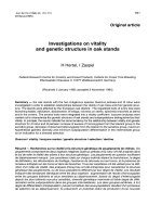
contains one locus only. Running Gene Stacker with any
preset and γ = 0.95 resulted in the schedule from
Figure 4 (left) which performs a single crossing. It is possible to immediately obtain the ideotype from this crossing
because the order of haplotypes within a chromosome
is arbitrary. This is taken into account when computing the probability of observing a genotype among the
offspring (Additional file 1: Section 1). In contrast, previous methods used a single chromosome and specified a
recombination rate of 0.5 between loci that actually reside
on different chromosomes. This requires to arbitrarily
fix an order of haplotypes in each actual chromosome
and artificially increases the complexity of the problem.
Figure 4 (right) shows Gene Stacker’s solution for the
same example when combining all loci on a single artificial chromosome. This schedule is significantly worse:
it has an additional generation and a much higher total
population size. Although this example was specifically
constructed and is somewhat extreme in the sense that
it has six loci on six different chromosomes, it clearly
shows the general benefits of explicitly modelling multiple
chromosomes.
Dealing with tight constraints

Tight constraints might apply for specific crops. For example, cotton plants can be used for two crossings only
(or one selfing) and each crossing yields a small amount
of about 250 seeds. This makes it more difficult to find
good crossing schedules within the constraints. With the

extended model such important constraints can easily
be taken into account. Crossings are performed multiple times if necessary to provide a sufficient amount of
seeds, where sometimes several duplicates of the same
genotype are needed to be able to make all crossings.
Population sizes are computed in such way that at least
the required number of duplicates of each targeted genotype is expected among the offspring (Additional file 1:
Section 2).
An example from cotton is considered with 6 parental
genotypes, 11 loci spread across 5 chromosomes and
a heterozygous ideotype (full description in Additional
file 1: Section 7). An overall success rate of γ = 0.95 was
used and the number of generations, number of plants per
generation and overall linkage phase ambiguity were limited to 5, 5000 and 10%, respectively. A time limit of 24
hours was applied. The number of crossings per plant and
seeds obtained per crossing were set to 2 and 250, respectively, to precisely reflect the tight constraints of cotton
breeding.
Running Gene Stacker with preset fastest took 2 hours
and 15 minutes to complete and reported 4 solutions with
3–5 generations, a total population size of 7256–1077 and
an overall linkage phase ambiguity of 0–3.14% (Additional
file 1: Figures S5–S8). All other presets ran out of memory (64 GB). When restricting the number of generations
to 4 instead of 5, preset faster reported a different solution
with 4 generations that has a lower total population size
(1400) than the respective schedule found by preset fastest
(1534) before being interrupted when the time limit of 24
hours had been exceeded (Additional file 1: Figure S9). All
solutions contain at least one crossing which is performed
multiple times and/or a genotype of which multiple duplicates are selected. It was not possible to obtain solutions
within the constraints using CANZAR as this method
does not provide a way to accurately impose and work

around these constraints.
Optimization power and heuristics

We first explore the limits of the optimization strategy
and the power gained by applying additional heuristics,
based on experiments with a large number of randomly
generated problem instances. Then, the obtained qualityruntime tradeoff is assessed for various complex, real
stacking problems.
Limits of the optimization strategy

Experiments have been performed with a variety of
240 randomly generated stacking problems; 120 with a
homozygous ideotype and 120 with a heterozygous ideotype. All instances have 4–14 loci, taking steps of two,
and 20 instances were created for every number of loci
and for both types of ideotype. Each instance has been
independently generated by


De Beukelaer et al. BMC Genetics (2015) 16:2

Page 11 of 16

S1

S2

1

1

[0 0 0 0 0 0]
[0 1 1 1 1 1]

[0 0 0 0 0 0]
[1 1 1 1 1 0]

S2

S1

1

1
[0][0][0][0][0][0]
[1][1][1][1][1][0]

[0][0][0][0][0][0]
[0][1][1][1][1][1]

S3

4174
[0 0 0 0 0 0]
[0 0 0 0 0 0]

[0 1 1 1 1 1]
[1 1 1 1 1 0]

S3

191
[0][0][0][0][0][0]
[1][1][1][1][1][1]

S4

15
Overall LPA: 0%
# Plants: 193

[0 0 0 0 0 0]
[1 1 1 1 1 1]

Overall LPA: 0%
# Plants: 4191

Figure 4 Solutions for second constructed example. (left) Best solution obtained for the second constructed example when explicitly modelling
multiple chromosomes; (right) best solution found when combining all loci on one artificial chromosome, where a crossover rate of 0.5 is specified
between pairs of consecutive loci that actually reside on different chromosomes (in this example, all loci).

(i) picking a random number of 1–8 chromosomes,
limited by the number of loci;
(ii) randomly assigning each locus to one of the available
chromosomes, with a minimum of 1 locus per
chromosome;
(iii) setting a random distance of 1–50 cM between pairs
of consecutive loci on the same chromosome;
(iv) randomly creating 2–8 parental genotypes, where
each allele is set to 1 or 0 with equal probability; and
(v) generating a random ideotype.

The haplotypes of the ideotype’s chromosomes were
created by copying alleles from one of both haplotypes of
the respective chromosome of a randomly picked parental
genotype (independently for every locus). To obtain a
homozygous ideotype, one haplotype is created for each
chromosome and included twice. For heterozygous ideotypes, two independent haplotypes are created and combined for every chromosome.
Figure 5 shows results of running each preset of Gene
Stacker on the 120 instances with a homozygous ideotype.
All experiments have been repeated with a maximum of
4, 5 and 6 generations, and a runtime limit of 24 hours

has been applied, together with an overall success rate of
γ = 0.95 and a maximum of 10000 plants per generation,
4 crossings per plant, 5000 obtained seeds per crossing
and 20% overall linkage phase ambiguity. For every combination of the maximum number of generations (rows), the
number of loci (columns) and the applied preset (bars) it
is reported for how many out of 20 instances Gene Stacker
completed within the time limit of 24 hours.
Without applying any heuristics (preset best), Gene
Stacker solves only 42.5%, 35% and 28.34% of all instances
when limiting the number of generations to 4, 5 and
6, respectively. Interestingly, solutions are obtained for
about 95% of all instances when applying all heuristics
(preset fastest) regardless of the limit on the number
of generations. As expected (and desired), the power of
the other presets (better, default, faster) lies somewhere
in between. The problem complexity obviously increases
with the number of loci as well as the maximum number of generations. Without any heuristics, Gene Stacker
solved almost no problems with more than 8 loci: solutions were obtained for less than half of the instances
when the number of loci exceeded 8, 6 and 4 with a limit

of 4, 5 and 6 generations, respectively. Yet, Gene Stacker


De Beukelaer et al. BMC Genetics (2015) 16:2

Page 12 of 16

Figure 5 Results for random instances with a homozygous ideotype. This figure indicates the number of randomly generated instances with a
homozygous ideotype for which the different presets of Gene Stacker completed within the applied time limit of 24 hours. Experiments were
repeated with a maximum of 4–6 generations. Instances have 4–14 loci spread across 1–8 chromosomes and 2–8 parental genotypes. In total, 20
instances were generated for each number of loci.

can cope with many more complex problems with up to
at least 14 loci using the proposed heuristics. Of course,
these heuristics may yield worse Pareto frontier approximations, so it is preferred only to enable them if necessary
to find solutions within reasonable time. In this way, the
heuristics offer a convenient quality-runtime tradeoff and
allow to obtain (approximate) solutions for more complex
problems.

Figure 6 shows similar results for the 120 instances with
a heterozygous ideotype. It is clear that these are generally more complex as significantly fewer instances were
solved within the time limit compared to the results from
Figure 5. This may be explained from the fact that each
heterozygous chromosome in the ideotype contains two
different target haplotypes, i.e. two competing goals, that
have to be obtained simultaneously. Also, the heuristics


De Beukelaer et al. BMC Genetics (2015) 16:2

Page 13 of 16

Figure 6 Results for random instances with a heterozygous ideotype. This figure indicates the number of randomly generated instances with a
heterozygous ideotype for which the different presets of Gene Stacker completed within the applied time limit of 24 hours. Experiments were
repeated with a maximum of 4–6 generations. Instances have 4–14 loci spread across 1–8 chromosomes and 2–8 parental genotypes. In total, 20
instances were generated for each number of loci.

are less effective for heterozygous ideotypes. For example, improvement towards any of both haplotypes of a
heterozygous ideotype chromosome is rewarded; therefore, heuristics based on such improvement are less powerful in case of two distinct target haplotypes in a single
chromosome.
Without applying any heuristics, Gene Stacker now
solves 22.5–37.5% of all instances for a varying limit on
the number of generations. Less than half of the instances

were solved when the number of loci exceeded 4–6. When
all heuristics are enabled, solutions are obtained for 65–
72.5% of the instances (for less than half of the instances
when exceeding 10 loci). Although the currently proposed
heuristics are clearly less powerful when aiming for a
heterozygous ideotype, they allowed to find solutions for
many complex problems with up to 10 loci. Nevertheless,
the challenge remains to develop better heuristics in this
respect.


De Beukelaer et al. BMC Genetics (2015) 16:2

We conclude that the applied optimization strategy can
effectively be used to find solutions for a wide range of

stacking problems. Without extra heuristics, some smaller
problems with 4–8 or 4–6 loci in case of a homozygous or
heterozygous ideotype, respectively, can already be tackled (depending on the maximum number of generations).
To deal with more complex problems, additional heuristics are required. The proposed heuristics allow to obtain
(approximate) solutions for problems with up to at least
10–14 loci.
Quality-runtime tradeoff

The quality-runtime tradeoff obtained by applying different combinations of heuristics is assessed here for real
stacking problems from tomato and rice (full specification in Additional file 1: Section 7). For all experiments, an
overall success rate of γ = 0.95 was set and the number
of generations and plants per generation were restricted
to 5 and 5000, respectively. The amount of seeds produced per crossing and maximum number of crossings
per plant were set to reflect the specific properties of each
crop. Approximated Pareto frontiers in terms of the total
population size and number of generations are reported
(only schedules with zero linkage phase ambiguity were
selected).
First, experiments were performed with two stacking
problems from tomato. Both consist of the same 4 parental
genotypes with 8 loci spread across 6 chromosomes. The
first example (Tomato-1) has a homozygous ideotype
while the second example (Tomato-2) has a heterozygous
ideotype. Tomatoes can easily be crossed several dozens
of times and every crossing yields a large number of seeds:
the maximum number of crossings per plant and the
amount of seeds obtained from one crossing were set to
24 and 20000, respectively. A time limit of 12 hours was
imposed, after which the algorithms were interrupted and
the solutions found until then were inspected.

Figure 7 (top left) shows the Pareto frontier approximations obtained by applying Gene Stacker with presets
default, faster and fastest as well as CANZAR to Tomato1. Gene Stacker and CANZAR obtained exactly the same
schedule with 4 generations. The small difference in the
reported population size is explained by the fact that both
methods follow a slightly different approach to derive a
success rate per targeted genotype (γ ) from the desired
overall success rate (γ ). Solutions with 5 generations were
also found. Those reported by Gene Stacker have a lower
population size compared to the one obtained by CANZAR, even when applying preset fastest which completes
after only 28 seconds. Presets default and faster reported
exactly the same solutions and the 5 generation schedule found here improves over the respective schedule
obtained by preset fastest. Yet, these two presets took significantly more time (ca. 6–8 hours). This shows how the

Page 14 of 16

proposed heuristics provide tradeoffs between solution
quality and execution time and that they are capable of
finding good solutions for a complex, realistic problem
within reasonable time. CANZAR was interrupted when
exceeding the time limit of 12 hours.
Similar results for Tomato-2 are presented in Figure 7
(top right) where only preset fastest has been applied
since the other presets ran out of memory (64 GB). Gene
Stacker completed in about 5 hours while CANZAR was
interrupted when the time limit had expired. Three solutions were reported by Gene Stacker with 3–5 generations
and CANZAR obtained 2 solutions with 4–5 generations.
The 4 generation schedules reported by both methods
slightly differ but have approximately the same total population size. Conversely, Gene Stacker found a somewhat
better schedule with 5 generations and an additional solution with only 3 generations. The difference in runtime, as
compared to Tomato-1, and the fact that all other presets

ran out of memory again confirm that with the current
heuristics it is more difficult to solve stacking problems
with a heterozygous ideotype. Yet, the heuristics made it
possible to find 3 good solutions within a few hours, using
a transparent optimization strategy.
Results were also obtained for two examples from rice.
Both consist of the same 8 parental genotypes with 10 loci
spread across 6 chromosomes. The first example (Rice1) has a homozygous ideotype while the second example
(Rice-2) has a heterozygous ideotype. About 300 seeds
are obtained from each crossing and rice plants can be
crossed no more than 5 times. For these examples, a time
limit of 24 hours was set.
Figure 7 (bottom left) shows the Pareto frontier approximations obtained by applying Gene Stacker with presets
better, default, faster and fastest as well as CANZAR
to Rice-1. Preset fastest completed after only 4 seconds
and reported three solutions with 3–5 generations. Presets default and faster terminated after about 30 seconds and found a better schedule that dominates both
the 4 and 5 generation schedules obtained by preset
fastest. Preset better completed after about 12 minutes
and found an additional 5 generation schedule with a
slightly lower total population size. This again shows how
the heuristics offer a convenient quality-runtime tradeoff. CANZAR did not complete within the time limit
of 24 hours but was able to obtain a single schedule
with 4 generations that dominates all 4 and 5 generation schedules obtained by Gene Stacker. It is inevitable
that the heuristics sometimes make wrong decisions in
which case valuable parts of the search space may not
have been explored. In this specific example, heuristic
H0 (included in all presets except preset best) removed a
parental genotype that is needed to find the better schedule obtained by CANZAR. Still, results are quite close
to those of CANZAR, especially when applying presets

De Beukelaer et al. BMC Genetics (2015) 16:2

Page 15 of 16

Pareto frontier approximations (Tomato-1)

1325

Pareto frontier approximations (Tomato-2)

3250

Fastest (28s)
Default (7h 28m), Faster (6h 12m)
CANZAR (>12h, interrupted)

1300
1275

2750

1250
1225

Population size

Population size

Fastest (5h 8m)

CANZAR (>12h, interrupted)

3000

1200
1175
1150
1125
1100
1075

2500
2250
2000
1750
1500
1250

1050
1000

1025

750

1000
4

3

5

Number of generations

950

Fastest (4s)
Default (33s), Faster (28s)
Better (12m 17s)
CANZAR (>24h, interrupted)

Fastest (5m 36s)
CANZAR (>24h, interrupted)

900
850

Population size

Population size

5

Pareto frontier approximations (Rice-2)

Pareto frontier approximations (Rice-1)
600
575
550
525

500
475
450
425
400
375
350
325
300
275

4

Number of generations

800
750
700
650
600
550
500
450

3

4

5

Number of generations

3

4

5

Number of generations

Figure 7 Pareto frontier approximations of real stacking problems from tomato and rice. (top left) First example from tomato (Tomato-1),
homozygous ideotype; (top right) second example from tomato (Tomato-2), heterozygous ideotype; (bottom left) first example from rice (Rice-1),
homozygous ideotype; (bottom right) second example from rice (Rice-2), heterozygous ideotype. Full descriptions of the examples are provided in
the Additional file 1: Section 7.

faster, default or better, a significant speedup is obtained
and an additional solution with only 3 generations is
found.
Similar results for Rice-2 are shown in Figure 7 (bottom
right) where only preset fastest has been applied as the
other presets either ran out of memory or did not find
any solutions within the time limit. Gene Stacker completed after 5–6 minutes while CANZAR was interrupted
after exceeding the time limit of 24 hours. Three solutions
were reported by Gene Stacker, with 3–5 generations.
CANZAR found a single solution with 4 generations and
a higher population size than the respective schedule
obtained by Gene Stacker. Again, the runtime and memory footprint of Gene Stacker is significantly higher for
this problem with a heterozygous ideotype as compared
to Rice-1 which has a homozygous ideotype. Yet, preset
fastest outperforms CANZAR and is able to provide a

valuable approximation of the Pareto frontier within a few
minutes.

Practical guidelines

Based on our findings we propose the following practical guidelines for using Gene Stacker. Best is to first
try the default settings, specifying the required parameters (maximum number of generations and overall success
rate) and those constraints that are important for the specific application (such as the number of seeds produced
from a crossing and maximum number of crossings per
plant) with a reasonable runtime limit (e.g. 24 hours). If
Gene Stacker is too slow or requires too much memory, consider setting additional or tighter constraints (e.g.
maximum plants per generation, maximum overall linkage phase ambiguity, ...) and/or using preset faster or
fastest. The latter may yield worse solutions which should
be avoided when possible. In case the default setting is
more than fast enough consider running presets better
and best as well to check whether this produces better
schedules, as the heuristics might have missed something. Usually, differences between the latter presets and


De Beukelaer et al. BMC Genetics (2015) 16:2

the default setting are very small (if any) except for the
runtime which is significantly increased.
In case QTL (quantitative trait locus) intervals need to
be stacked one can use flanking markers to delimit the
target locus. The Tomato-1 problem (Additional file 1:
Section 7) is a case in point. On the sixth chromosome, a
small region of 10 cM has been identified in which a target gene is located. In this setting it is advised to make
sure that the required haplotype is present in at least one
of the parents, and to verify it is maintained throughout

the crossing scheme. There always remains a small risk of
a double cross-over within the interval in a single generation which one can either ignore or monitor by saturating
the interval with additional markers. More details and
practical examples are given at .

Conclusions
The proposed transparent, flexible and easily extensible
approach to marker-assisted gene pyramiding was confirmed to be feasible in combination with heuristics to
address realistic, complex stacking problems with up to
at least 10–14 loci, while taking into account important
breeding constraints. Carefully designed heuristics even
allow to find better or additional solutions within reasonable time compared to previous methods. The proposed
heuristics are certainly not perfect nor complete. For
example, they are less effective for problems with a heterozygous ideotype. Future work may include the design
of additional or improved heuristics as well as extension
of the ideas applied in Gene Stacker for a more general
plant breeding context that also addresses complex traits
and conservation of genetic background.

Availability of supporting data
The data set(s) supporting the results of this article is(are)
included within the article (and its additional file(s)).

Endnotes
a
See .
b
The term ‘homozygous genotype’ is used to indicate
that all considered loci are homozygous; this does not say
anything about the remaining loci in the full DNA and

should for example not be confused with homozygous
inbred lines.
c
Experiments with CANZAR were run on the SURFsara
Lisa computing system ( />systems/lisa/description) by the authors of this method.
Additional file
Additional file 1: Supplementary material. PDF file with supplementary
information such as formulas, algorithm details and additional results.

Page 16 of 16

Abbreviations
MIP: Mixed integer programming; DAG: Directed acyclic graph; LPA: Linkage
phase ambiguity; QTL: Quantitative trait locus.
Competing interests
HDB and VF declare that they have an ongoing scientific collaboration with
Bayer CropScience where GDM is employed. VF has also been involved in
consultancy for this company.
Authors’ contributions
HDB proposed the Gene Stacker algorithm, implemented it and performed all
experiments under the supervision of VF. GDM provided data, general advice
on the genetical context and assistance for the development of heuristics.
HDB wrote the initial manuscript with all authors contributing to the final
version. All authors read and approved the final manuscript.
Acknowledgements
This work was carried out using the Stevin Supercomputer Infrastructure at
Ghent University. We thank Mohammed El-Kebir and Stefan Canzar for their
kind cooperation by running their algorithm on our test cases. This allowed for
an interesting comparison between our methods and made a major
contribution to the discussion. Herman De Beukelaer is supported by a Ph.D.

grant from the Research Foundation of Flanders (FWO).
Author details
1 Department of Applied Mathematics, Computer Science and Statistics, Ghent
University, Krijgslaan 281 - S9, 9000 Gent, Belgium. 2 Bayer CropScience NV,
Innovation Center, Technologiepark 38, 9052 Zwijnaarde, Belgium.
Received: 19 September 2014 Accepted: 16 December 2014

References
1. Tester M, Langridge P: Breeding technologies to increase crop
production in a changing world. Science 2010, 327(5967):818–22.
2. Moose SP, Mumm RH: Molecular plant breeding as the foundation for
21st century crop improvement. Plant Physiol 2008, 147(3):969–77.
3. de los Campos G, Hickey JM, Pong-Wong R, Daetwyler HD, Calus MP:
Whole-genome regression and prediction methods applied to plant
and animal breeding. Genetics 2013, 193(2):327–45.
4. Ishii T, Yonezawa K: Optimization of the marker-based procedures for
pyramiding genes from multiple donor lines: I. schedule of crossing
between the donor lines. Crop Sci 2007, 47(2):537–546.
5. Ye G, Smith KF: Marker-assisted gene pyramiding for inbred line
development: Basic principles and practical guidelines. Int J Plant
Breed 2008, 2(1):1–10.
6. Servin B, Martin OC, Mézard M, Hospital F: Toward a theory of
marker-assisted gene pyramiding. Genetics 2004, 168:513–23.
7. Xu P, Wang L, Beavis WD: An optimization approach to gene stacking.
Eur J Oper Res 2011, 214:168–78.
8. Canzar S, El-Kebir M: A mathematical programming approach to
marker-assisted gene pyramiding. In Algorithms in Bioinformatics, WABI
2011, LNBI 6833. Edited by Przytycka TM, Sagot M.-F. Berlin, Germany:
Springer; 2011:26–38.
9. Haldane J: The combination of linkage values and the calculation of

distances between the loci of linked factors. J Genet 1919,
8(29):299–309.
10. Browning SR, Browning BL: Haplotype phasing: existing methods and
new developments. Nat Rev Genet 2011, 12(10):703–14.
11. El-Kebir M, de Berg M, Buntjer J: Crossing schedule optimization.
[Master’s thesis]. Technische Universiteit Eindhoven; 2009.