0202zuzarte

Partitioning in DB2 Using the UNION ALL View
Calisto Zuzarte Robert Neugebauer Natt Sutyanyong Xiaoyan Qian Rick Berger
IBM Toronto IBM Toronto IBM Toronto IBM Toronto IBM Boca Raton
© Copyright International Business Machines Corporation 2002. All rights reserved.
Abstract
In today’s relational databases, it is not uncommon to hear of terabyte-size databases. As it becomes
necessary to store ever increasing volumes of data in a single table within the database, more people need
to know how to manage this data. The solution to many of these situations is typically one of ”divide and
conquer.” The commonly recommended solution when using DB2® Universal Database™ Version 7 on the
various workstation platforms is to use a partitioned database. While it is well recognized that there needs
to be other long term solutions, this paper discusses an existing “partitioning” solution—namely, the
approach of using a UNION ALL view. The treatment of the UNION ALL view in the DB2 query rewrite
component of the DB2 SQL compiler has been sufficiently enhanced to make it worth considering when
there is a requirement to manage data that is large but needs to be viewed as a single relation.
Contents
1. Introduction...................................................................................................................................2
2. A business application and possible database Issues....................................................................2
3. Using a UNION ALL view...............................................................................................................3
4. DB2 query rewrite and the UNION ALL view..................................................................................5
4.1 Local predicate pushdown...........................................................................................................6
4.2 Redundant branch elimination......................................................................................................7
4.3 Join pushdown.........................................................................................................................10
4.4 GROUP BY pushdown..............................................................................................................13
4.5 The result of the query rewrite transformations.............................................................................14
4.6 Runtime branch elimination with parameter markers....................................................................16
5. Benefits of UNION ALL views......................................................................................................18
5.1 Better control of maintenance window utilities..............................................................................19
5.2 Easier to roll data in and out......................................................................................................19
5.3 Ability to leverage different storage media....................................................................................20
5.4 More granular performance tuning...............................................................................................20
5.5 Easier to modify the schema and the data...................................................................................20

5.6 Decreased I/O costs..................................................................................................................22
5.7 Increased query parallelism........................................................................................................22
5.8 Optimizing UNION ALL Views in a federated environment...............................................................23
6. Limitations of using UNION ALL views........................................................................................23
6.1 Risk of view materialization with complex queries.........................................................................23
6.2 Problems guaranteeing uniqueness across tables in a view...........................................................23
6.3 Restrictions on inserting into a UNION ALL view...........................................................................24
6.4 Limitations on the number of branches in a UNION ALL view.........................................................24
6.5 Increased compile time and memory usage.................................................................................24
6.6. Future enhancements.................................................................................................................25
7. Conclusion...................................................................................................................................25
Page 1 of 25
1. Introduction
Business intelligence applications that are used today require that large amounts of historical data be
stored. One common application is to store and analyze prior business transactions, such as sales data,
over a period of several years. It is easy to envision a sales forecasting system that stores all sales
transactions for three years with 500 MB of data generated daily. That would require active storage of
approximately 500 GB of data just for sales.
Early versions of DB2 were limited to storing data in table spaces consisting of 4KB pages. With these 4KB
pages, an individual row within a table uses a four-byte row identifier (RID) to locate a row. Of these four
bytes, three are used to identify a page and one to identify the offset within a page. The maximum number of
pages was therefore limited by the maximum integer that could be stored in 3 bytes. So with 16 million
4KB pages, the limit for a single table was 64 GB. Subsequent versions of DB2 introduced larger page sizes
that allowed this limit to be stretched to 512 GB by using a 32KB page size table space. Yet, as the
example in the previous paragraph showed, this limit was a problem. Other than not having enough room to
define indexes and other tables, there was no room to grow.
To overcome these table size limits and to achieve scalability through parallelism, DB2 adopted a
shared-nothing architecture in 1995. This partitioned database allowed the table to be partitioned on several
nodes of a cluster or within a single SMP server where each partition had the table size limits. The size of
the table could now be extended depending on how many partitions could be provided. The partition ID

extended the RID to allow for much more data to be stored in the table. The data is distributed among
various partitions using a hash partitioning scheme by hashing the values of one or more columns in the
table. This is the general recommendation to overcome the size limits of a table in DB2.
There might be a situation when a single-partition DB2 user has not anticipated the growth of a table or does
not want to move to a partitioned database in the near time frame. One approach that might be worth
considering is instead of storing the data in a single table, use a UNION ALL view over multiple tables.
Application queries can refer to this view to look at the data in all the component tables as a single entity.
The purpose of this paper is to discuss the advantages and disadvantages of this approach.
This paper is organized as follows.
Ÿ Section 2 introduces a typical business application and possible database issues.
Ÿ Section 3 presents the approach of using a UNION ALL view to solve these related issues.
Ÿ Section 4 describes the work done by the query rewrite component of the SQL compiler in DB2 in order
to optimize the query. Each type of optimization is explored in detail, laying out the evolution of a query.
Finally, the optimized query is compared with the original query.
Ÿ Sections 5 and 6 describe the benefits and limitations of using a UNION ALL view, respectively.
Ÿ Section 7 is a conclusion.
2. A business application and possible database issues
A worldwide trading company has decided to create a data warehouse for its sales data. The finance
department wants to track and analyze the sales revenue across geographies for all products sold on a
periodic basis. The logical design of the tables is as follows.
sales( sales_date date not null,
prod_id integer,
city_id integer,
channel_id integer,
revenue decimal(20,2))
Page 2 of 25
products(prod_id integer,
prod_desc varchar(50),
prod_group_id integer,
prod_group_desc varchar(50),

launch_date date,
terminated char(1))
geographies( region_id integer,
region varchar(50),
country_id integer,
country varchar(50),
state_id char(3),
state varchar(50),
city_id integer,
city varchar(50))
channel( channel_id integer,
channel varchar(50),
channel_cost decimal(20,2))
The sales table stores sales transactions over a period of three years. It is estimated that the sales
transactions collected from all the sales worldwide can be as large as 500 MB daily. The products table
records all products manufactured. The geographies table references a city_id to its corresponding city
name, state, country, and region. The channel table refers to all the channels the company uses to sell its
products and a consolidated channel cost.
With daily sales transactions of 500 MB, the sales table can grow to an approximate size of 15 GB in a
month and 180 GB in a year. On a single-partition database, it will take just three years of data to reach the
limits of the table. This could be a problem if, for whatever reason, moving to a partitioned database is
inappropriate. The first problem is the ability to store such large amounts of data given the single partition
limits required by this particular trading company.
Query performance on this table may be a concern. Indexes on the table could have more levels than those
on a smaller table. If there are many probes of the index, the extra disk I/O to navigate through the index
may not offer the best performance.
3. Using a UNION ALL view
Other than a multi-partitioned database, a practical approach to deal with the size of table and to manage
administration tasks is to physically partition the sales table into a set of smaller tables. In particular, the
sales table can be represented by tables of the same column definition but with each of the tables

representing different period of the sales transactions. For example, we may have table sales_0198 for sales
transactions in January 1998, table sales_0298 for transactions in February 1998 and so on. Then we “glue”
all the tables together as a view named all_sales using the UNION ALL construct. We will refer to this kind
of view as a UNION ALL view. Branches of the UNION ALL view do not need to have a uniform structure or
range of data. This allows complete customization based on performance and hardware characteristics.
One way of distributing the data could be done as follows:
Ÿ Data for the oldest year can be put in a single base table.
Ÿ Data for each quarter of the middle year can be put into separate tables.
Ÿ Finally, a single base table can be created for each month of the current year.
Page 3 of 25
The view can be named sales so that applications need not be changed.
In order to guarantee that the table sales_0198 will contain only sales transactions from January 1998, we
need to put a check constraint in the definition of the table as follows. Check constraints ensure that the
data integrity is maintained in accordance with the definition of the constraint.
create table sales_0198(
sales_date date not null,
prod_idinteger,
city_id integer,
channel_id integer,
revenuedecimal(20,2),
constraint ck_date
check
(sales_date between ‘01-01-1998’ and ‘31-01-1998’))
The check constraint is also necessary for DB2 query rewrite to improve the performance of the query
against the all_sales view by ensuring that only the relevant monthly sales tables are accessed, as is
described in more detail in Section 4.
Another option to achieve the same result is to define a WHERE clause on every table in the UNION ALL
view. You can use this option if there is a screening process in place before data is loaded into the table to
ensure that data is loaded to the proper table.
The following statement shows the definition of the view all_sales:

create view all_sales as
(
select * from sales_0198
where sales_date between ‘01-01-1998’ and ‘31-01-1998’
union all
select * from sales_0298
where sales_date between ‘01-02-1998’ and ‘28-02-1998’
union all
...
union all
select * from sales_1200
where sales_date between ‘01-12-2000’ and ‘31-12-2000’
);
The optional WHERE clauses (shown in bold for identification) are needed only if the base tables do not
define check constraints for the date ranges of the sales transactions.
If you are familiar with Oracle’s partitioned view, you may be wondering why Oracle plans to withdraw
support of that feature. This feature in Oracle is based on the same principle of dividing the table, but it is
more limited in the associated structures defining the view. All tables must have similar schema and
indexes. It does not have the flexibility and independence associated with the basic UNION ALL approach.
Many of the benefits that can be obtained using the UNION ALL view approach discussed here are not
applicable to Oracle’s partitioned view. Presumably, due to the availability of Oracle’s range partition and
limitations of Oracle’s partitioned view, it is being phased out.
Page 4 of 25
4. DB2 query rewrite and the UNION ALL view
The DB2 query rewrite component of the SQL compiler is a powerful transformation engine. The
optimizations listed below are performed by the query rewrite component. This list of optimizations includes
only those that are explicitly relevant to UNION ALL views; there are many other optimizations that will
benefit most queries.
The DB2 query rewrite engine attempts to prune the number of tables that need to be accessed in the
processing of the query. The following optimizations work together to improve the performance of a query

over a UNION ALL view:
Ÿ Local predicate pushdown.
Ÿ Redundant branch elimination.
Ÿ Join pushdown.
Ÿ Group by pushdown.
For each of these optimizations, we describe
Ÿ The benefits of the optimization.
Ÿ The result of each optimization on a sample query.
Ÿ The measures that are in place to deal with any possible drawbacks.
Throughout Section 4, we show the evolution of a query for the business problem above.
Some information that a company might want to obtain is the total revenue per active product generated in
each city by all distribution channels during January and February of 2000. You can express this as follows:
Query 1:
select s.prod_id, p.prod_desc, g.city, c.channel,
sum(s.revenue) as “Total Revenue”
from products p, geographies g, channel c, all_sales s
where s.prod_id = p.prod_id and
s.city_id = g.city_id and
s.channel_id = c.channel_id and
s.sales_date between ‘01-01-2000’ and ‘29-02-2000’ and
P.terminated = ‘N’
group by s.prod_id, p.prod_desc, s.city_id, g.city, s.channel_id, c.channel
Page 5 of 25
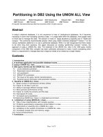
A graphical version of this query is depicted in Figure 1.
Select
Sales_0198 Sales_1200Sales_0298
...
Union View
(all_sales)
ChannelGeographies Products

Grouping
Figure 1. Graphical representation of Query 1
All of the optimization methods listed above can be applied to this query, and we will show in the following
sections how this query is transformed into its final form.
4.1 Local predicate pushdown
The DB2 query rewrite component pushes eligible local predicates down through SELECT, join, UNION, or
GROUP BY. The purpose of “predicate pushdown” is to apply the restrictions earlier to reduce the
intermediate data flows between operations. If the local predicates (ie., predicates not involving other tables)
can be pushed down to the operations at the lowest level when accessing the table, the restrictions made
by those predicates then will eliminate any unqualified rows and feed only the qualified rows to the next
upper level operations, and so on.
In the example query given in Section 4, there are three local predicates that are eligible to be pushed down:
‘01-01-2000’ <= s.sales_date, s.sales_date <= ‘29-02-2000’, and p.terminated =
‘N’. These two predicates that involve s.sales_date are pushed through the UNION ALL to each of the
partitioned sales tables; the predicate that involves p.terminated is pushed to the products table.
After local predicate pushdown, the query looks like this :
Query 2:
with p1 as (select prod_id, prod_desc from products
where terminated = ‘N’),
s1 as (select * from sales_0198
where ‘01-01-2000’ <= sales_date and sales_date <= ‘29-02-2000’),
s2 as (select * from sales_0298
where ‘01-01-2000’ <= sales_date and sales_date <= ‘29-02-2000’),
...
s36 as (select * from sales_1200
where ‘01-01-2000’ <= sales_date and sales_date <= ‘29-02-2000’),
sales2 as(select * from s1
union all
select * from s2
union all

Page 6 of 25
...
select * from s36)
select s.prod_id, p.prod_desc, g.city, c.channel, sum(s.revenue) as “Total
Revenue”
from p1 p, geographies g, channel c, sales2 s
where s.prod_id = p.prod_id and
s.city_id = g.city_id and
s.channel_id = c.channel_id
group by s.prod_id, p.prod_desc, s.city_id, g.city, s.channel_id, c.channel
The predicate is pushed down to all the base tables of the UNION ALL view all_sales as depicted in Figure
2.
'01-01-2000' <= sales_date
sales_date <= '29-02-2000'
'01-01-2000' <= sales_date
sales_date <= '29-02-2000'
'01-01-2000' <= sales_date
sales_date <= '29-02-2000'
Select
Select - S1 Select - S36Select - S2
...
Sales_0198 Sales_1200Sales_0298 ...
Products
ChannelGeographiesUnion All Select - P1
terminated='N'
Grouping
Figure 2. Graphical representation of Query 2
The benefit of applying predicates early is that the number of rows can be reduced earlier. In Query 2, we
are now filtering the rows from the products table and the UNION ALL view before the join. Assume that the
products table has 30,000 rows, but that only 1000 of them meet the condition terminated=’N’. Any join

that involves the products table will now be more efficient because there are fewer rows to join, and DB2
does not need to eliminate a substantial amount of rows from the result of the join.
4.2 Redundant branch elimination
This optimization method works in combination with local predicate pushdown to improve query
performance. Redundant branch elimination works by detecting inconsistencies in the predicate set for each
branch. If a given subset of the predicates is inconsistent, there is no way that the operation of that branch
will return any rows. If this branch of the UNION ALL view is removed, it will not affect the result of the query.
Page 7 of 25
Let us take a look at the created view S1. The predicates shown in bold are the check constraints defined
on the base table sales_0198.
Query 3:
select * from sales_0198
where ‘01-01-2000’ <= sales_date and
sales_date <= ‘29-02-2000’
and ‘01-01-1998’ <= sales_date and sales_date <= ‘31-01-1998’
It is not difficult to prove that there are no rows that satisfy all the four predicates in the SQL statement
above. Specifically, sales_date stored in table sales_0198 cannot be smaller than 01-01-98 and
simultaneously larger than 01-01-2000. When the DB2 optimizer detects this inconsistency, it knows that
this branch of UNION ALL does not need to be accessed and can be dropped from the UNION ALL view
even before executing the query. After eliminating the redundant branch, Query 2 in section 4.1 now looks
like this:
Query 4:
with p1 as (select prod_id, prod_desc from products
where terminated = ‘N’),
s25 as (select * from sales_0100
where ‘01-01-2000’ <= sales_date and sales_date <= ‘29-02-2000’),
s26 as (select * from sales_0200
where ‘01-01-2000’ <= sales_date and sales_date <= ‘29-02-2000’),
sales2 as(select * from s25
union all

select * from s26)
select s.prod_id, p.prod_desc, g.city, c.channel,
sum(s.revenue) as “Total Revenue”
from p1 p, geographies g, channel c, sales2 s
where s.prod_id = p.prod_id and
s.city_id = g.city_id and
s.channel_id = c.channel_id
group by s.prod_id, p.prod_desc, s.city_id, g.city, s.channel_id, c.channel
This is shown graphically in Figure 3. As you can see, the number of branches in the UNION ALL view has
been reduced from 36 to 2. There are now 34 fewer table or index accesses.
DB2 can detect inconsistencies most effectively with equality or inequality predicates (<, >, <=, >=, =, <>,
between); however, DB2 can also detect inconsistencies with more complicated predicate types, including
IN and OR predicates. With the more complicated predicate types, it might possibly be too difficult, too
expensive, or just not possible for DB2 to detect inconsistencies.
Page 8 of 25
Select
'01-01-2000' <= sales_date
sales_date <= '29-02-2000'
'01-01-2000' <= sales_date
sales_date <= '29-02-2000'
Select - S25
Sales_0100
Select - S26
Sales_0200
Products
ChannelGeographiesUnion All Select - P1
terminated='N'
Grouping
Figure 3. Graphical representation of Query 4
For example, if a query has multiple IN predicates, it requires comparing every element of each IN predicate.

This comparison is expensive to do, and IN predicates would not be inconsistent in most cases. DB2 does
make an exception when there is an equality predicate and an IN predicate. In that case, DB2 does do full
comparisons to detect inconsistencies.
For example, assuming that there is a UNION ALL view all_products for the products table that is
partitioned by the prod_group_id column. The view is set up so that each base table contains exactly one
product group and is enforced by an equality check constraint on prod_group_id. With this in place, the
following query is issued:
Query 5:
select * from all_product
where prod_group_id in (1, 3, 5)
DB2 can eliminate accesses to all base tables except the ones with prod_group_id as one of the elements
in the IN predicate.
Predicates that involve a function, e.g., UPPER(state) = ‘ONTARIO’, cannot be used to prove
inconsistency in order to eliminate branches (for reasons other than the fact that Ontario is a province and
not a state!). The exceptions are the YEAR and MONTH functions. For example, if the predicate
YEAR(sales_date)=2000 is specified, it would be converted to ‘01-01-2000’ <= sales_date
and sales_date < ‘01-01-2001’. Similarly, the predicates YEAR(sales_date)=2000 and
MONTH(sales_date)=2 can be converted to ‘01-02-2000’ <= sales_date and sales_date <
‘01-03-2000’. Attempting to use an IN predicate or an OR predicate along with the date function will fail
to enhance the pruning.
This is only an issue if the query predicates or check constraints use a function on the UNION ALL view
partitioning column. A solution to this is to use a generated column as the partitioning column. For example,
consider the table geographies that has a UNION ALL view defined over it using the state column as the
partitioning column. Ordinarily, branch elimination would not occur because of the UPPER function in the
Page 9 of 25
predicates. However, an uppercase representation of the state column could be generated and used as the
partitioning column for the UNION ALL view, as shown below:
create table geographies_1(
region_id integer,
region varchar(50),

country_id integer,
country varchar(50),
state_id char(3),
state varchar(50),
state_up generated always as (UPPER(state)),
city_id integer,
city varchar(50))
Query rewrite substitutes the predicate UPPER(state) = ‘ONTARIO’ with state_up = ‘ONTARIO’,
thus allowing branch elimination.
In DB2 Version 7, it is not always possible to remove branches from the access plan at compile time. There
are some situations where DB2 query rewrite introduces special execution time predicates that it evaluates
upfront to see if it needs to access a branch or not. This is not a bad thing and works well in some
situations, such as when parameter markers are present.
4.3 Join pushdown
For a UNION ALL view, the DB2 SQL optimizer tries to perform the “join pushdown” to the base tables.
Without pushing down the joins or the join predicates, DB2 would need to materialize the UNION ALL view
and then do the join. Join pushdown ensures that any indexes on the base tables are available to make the
join operation more efficient. This pushdown of joins usually has the same benefit as local predicate
pushdown because it may reduce the number of rows flowing to upper operations. The join pushdown is
limited to equi-join predicates only and when the number of the remaining branches in the UNION ALL view
is less than 36. These limits will be revised upwards in future versions of DB2. Join pushdown is applied after
any redundant branch elimination has occurred.
Let’s return to the example from Section 4. After join pushdown, Query 4 looks like this:
Query 6:
with s25 as (select s.prod_id, p.prod_desc, g.city, c.channel, s.revenue
from sales_0100 s, products p, geographies g, channel c
where ‘01-01-2000’ <= sales_date and sales_date <= ‘29-02-2000’ and
s.prod_id = p.prod_id and
s.city_id = g.city_id and
s.channel_id = c.channel_id and

p. terminated = ‘N’),
s26 as (select s.prod_id, p.prod_desc, g.city, c.channel, s.revenue
from sales_0200 s, products p, geographies g, channel c
where ‘01-01-2000’ <= sales_date and sales_date <= ‘29-02-2000’ and
s.prod_id = p.prod_id and
s.city_id = g.city_id and
s.channel_id = c.channel_id and
p. terminated = ‘N’),
sales2 as (select * from s25
union all
select * from s26)
Page 10 of 25