discriminative random fields- a discriminative framework for contextual interaction in classification
Bạn đang xem bản rút gọn của tài liệu. Xem và tải ngay bản đầy đủ của tài liệu tại đây (239.29 KB, 8 trang )
Discriminative Random Fields: A Discriminative Framework for Contextual
Interaction in Classification
Sanjiv Kumar and Martial Hebert
The Robotics Institute, Carnegie Mellon University
Pittsburgh, PA 15213, USA, {skumar, hebert}@ri.cmu.edu
Abstract
In this work we present Discriminative Random Fields
(DRFs), a discriminative framework for the classification of
image regions by incorporating neighborhood interactions
in the labels as well as the observed data. The discrimi-
native random fields offer several advantages over the con-
ventional Markov Random Field (MRF) framework. First,
the DRFs allow to relax the strong assumption of condi-
tional independence of the observed data generally used in
the MRF framework for tractability. This assumption is too
restrictive for a large number of applications in vision. Sec-
ond, the DRFs derive their classification power by exploit-
ing the probabilistic discriminative models instead of the
generative models used in the MRF framework. Finally, all
the parameters in the DRF model are estimated simulta-
neously from the training data unlike the MRF framework
where likelihood parameters are usually learned separately
from the field parameters. We illustrate the advantages of
the DRFs over the MRF framework in an application of
man-made structure detection in natural images taken from
the Corel database.
1. Introduction
The problem of region classification, i.e. segmentation
and labeling of image regions is of fundamental interest
in computer vision. For the analysis of natural images, it
is important to use the contextual information in the form
of spatial dependencies in the images. Markov Random
Field (MRF) models have been used extensively for vari-
ous segmentation and labeling applications in vision, which
allow one to incorporate contextual constraints in a princi-
pled manner [15].
MRFs are generally used in a probabilistic generative
framework that models the joint probability of the observed
data and the corresponding labels. In other words, let y be
the observed data from an input image, where y = {y
i
}
i∈S
,
y
i
is the data from the i
th
site, and S is the set of sites.
Let the corresponding labels at the image sites be given by
x = {x
i
}
i∈S
. In the MRF framework, the posterior over
the labels given the data is expressed using the Bayes’ rule
as,
P (x|y) ∝ p(x, y) = P (x)p(y|x)
where the prior over labels, P(x) is modeled as a MRF.
For computational tractability, the observation or likeli-
hood model, p(y|x) is assumed to have a factorized form,
i.e. p(y|x) =
i∈S
p(y
i
|x
i
) [1][4][15][22]. However, as
noted by several researchers [2][13][18][20], this assump-
tion is too restrictive for several applications in vision. For
example, consider a class that contains man-made structures
(e.g. buildings). The data belonging to such a class is highly
dependent on its neighbors. This is because, in man-made
structures, the lines or edges at spatially adjoining sites fol-
low some underlying organization rules rather than being
random (See Figure 1 (a)). This is also true for a large num-
ber of texture classes that are made of structured patterns.
In this work we have chosen the application of man-made
structure detection purely as a source of data to show the ad-
vantages of the Discriminative Random Field (DRF) model.
Some efforts have been made in the past to model the
dependencies in the data. In [11], a technique has been pre-
sented that assumes the noise in the data at neighboring sites
to be correlated, which is modeled using an auto-normal
model. However, the authors do not specify a field over
the labels and classify a site by maximizing the local poste-
rior over labels given the data and the neighborhood labels.
In probabilistic relaxation labeling, either the labels are as-
sumed to be independent given the relational measurements
at two or more sites [3] or conditionally independent in lo-
cal neighborhood of a site given its label [10]. In the context
of hierarchical texture segmentation, Won and Derin [21]
model the local joint distribution of the data contained in
the neighborhood of a site assuming all the neighbors from
the same class. They further approximate the overall likeli-
hood to be factored over the local joint distributions. Wil-
son and Li [20] assume the difference between observations
from the neighboring sites to be conditionally independent
given the label field.
In the context of multiscale random field, Cheng and
Bouman [2] make a more general assumption. They as-
sume the difference between the data at a given site and
the linear combination of the data from that site’s parents
to be conditionally independent given the label at the cur-
rent scale. All the above techniques make simplifying as-
sumptions to get some sort of factored approximation of the
likelihood for tractability. This precludes capturing stronger
relationships in the observations in the form of arbitrarily
complex features that might be desired to discriminate be-
tween different classes. A novel pairwise MRF model is
suggested in [18] to avoid the problem of explicit modeling
of the likelihood, p(y|x). They model the joint p(x, y) as
a MRF in which the label field P (x) is not necessarily a
MRF. But this shifts the problem to the modeling of pairs
(x, y). The authors model the pair by assuming the ob-
servations to be the true underlying binary field corrupted
by correlated noise. However, for most of the real-world
applications, this assumption is too simplistic. In our previ-
ous work [13], we modeled the data dependencies using a
pseudolikelihood approximation of a conditional MRF for
computational tractability. In this work, we explore alter-
native ways of modeling data dependencies which permit
eliminating these approximations in a principled manner.
Now considering a different point of view, for classifica-
tion purposes, we are interested in estimating the posterior
over labels given the observations, i.e., P(x|y). In a gener-
ative framework, one expends efforts to model the joint dis-
tribution p(x, y), which involves implicit modeling of the
observations. In a discriminative framework, one models
the distribution P (x|y) directly. As noted in [4], a poten-
tial advantage of using the discriminative approach is that
the true underlying generative model may be quite complex
even though the class posterior is simple. This means that
the generative approach may spend a lot of resources on
modeling the generative models which are not particularly
relevant to the task of inferring the class labels. Moreover,
learning the class density models may become even harder
when the training data is limited [19].
In this work we present a new model called Discrimi-
native Random Field based on the concept of Conditional
Random Field (CRF) proposed by Lafferty et al. [14] in
the context of segmentation and labeling of the 1-D text se-
quences. The CRFs directly model the posterior distribution
P (x|y) as a Gibbs field. This approach allows one to cap-
ture arbitrary dependencies between the observations with-
out resorting to any model approximations. CRFs have been
shown to outperform the traditional Hidden Markov Model
based labeling of text sequences [14]. Our model further
enhances the CRFs by proposing the use of local discrimi-
native models to capture the class associations at individual
sites as well as the interactions with the neighboring sites on
(a) Input image (b) DRF result
Figure 1. A natural image and the corresponding DRF re-
sult. A bounding square indicates the presence of struc-
ture at that block. This example is to illustrate the fact
that modeling data dependency is important for the de-
tection of man-made structures.
2-D lattices. The proposed DRF model permits interactions
in both the observed data and the labels. An example result
of the DRF model applied to man-made structure detection
is shown in Figure 1 (b).
2. Discriminative Random Field
We first restate in our notations the definition of the Con-
ditional Random Fields as given by Lafferty et al. [14]. As
defined before, the observed data from an input image is
given by y = {y
i
}
i∈S
where y
i
is the data from i
th
site and
y
i
∈
c
. The corresponding labels at the image sites are
given by x = {x
i
}
i∈S
. In this work we will be concerned
with binary classification, i.e. x
i
∈ {−1, 1}. The random
variables x and y are jointly distributed, but in a discrimina-
tive framework, a conditional model P (x|y) is constructed
from the observations and labels, and the marginal p(y) is
not modeled explicitly.
CRF Definition: Let G = (S, E) be a graph such that x is
indexed by the vertices of G. Then (x, y) is said to be a con-
ditional random field if, when conditioned on y, the random
variables x
i
obey the Markov property with respect to the
graph: P (x
i
|y, x
S−{i}
) = P (x
i
|y, x
N
i
), where S − {i} is
the set of all nodes in the graph except the node i, N
i
is the
set of neighbors of the node i in G, and x
Ω
represents the
set of labels at the nodes in set Ω.
Thus, a CRF is a random field globally conditioned on
the observations y. The condition of positivity requiring
P (x|y) > 0 ∀ x has been assumed implicitly. Now, using
the Hammersley Clifford theorem [15] and assuming only
up to pairwise clique potentials to be nonzero, the joint dis-
tribution over the labels x given the observations y can be
written as,
P (x|y)=
1
Z
exp
i∈S
A
i
(x
i
, y)+
i∈S
j∈N
i
I
ij
(x
i
, x
j
, y)
(1)
where Z is a normalizing constant known as the partition
function, and -A
i
and -I
ij
are the unary and pairwise po-
tentials respectively. With a slight abuse of notations, in
the rest of the paper we will call A
i
the association poten-
tial and I
ij
the interaction potential. Note that both terms
explicitly depend on all the observations y. Lafferty et al.
[14] modeled the association and the interaction potentials
as linear combinations of a predefined set of features from
text sequences. In contrast, we look at the association po-
tential as a local decision term which decides the associa-
tion of a given site to a certain class ignoring its neighbors.
In the MRF framework, with the assumption of conditional
independence of the data, this potential is similar to the log
likelihood of the data at that site. The interaction potential
is seen in DRFs as a data dependent smoothing function. In
the rest of the paper we assume the random field given in
Eq. (1) to be homogeneous and isotropic, i.e. the functional
forms of A
i
and I
ij
are independent of the locations i and j.
Henceforth we will leave the subscripts and simply use the
notations A and I. Note that the assumption of isotropy can
be easily relaxed at the cost of a few additional parameters.
2.1. Association Potential
In the DRF framework, A(x
i
, y) is modeled using a local
discriminative model that outputs the association of the site
i with class x
i
. Generalized Linear Models (GLM) are used
extensively in statistics to model the class posteriors given
the observations [16]. For each site i, let f
i
(y) be a function
that maps the observations y on a feature vector such that
f
i
: y →
l
. Using the logistic function as the link, the
local class posterior can be modeled as,
P (x
i
=1|y)=
1
1+e
−(w
0
+w
T
1
f
i
(y))
=σ(w
0
+w
T
1
f
i
(y))
(2)
where w = {w
0
, w
1
} are the model parameters. To extend
the logistic model to induce a nonlinear decision boundary
in the feature space, a transformed feature vector at each site
i is defined as, h
i
(y) = [1, φ
1
(f
i
(y)), . . . , φ
R
(f
i
(y))]
T
where φ
k
(.) are arbitrary nonlinear functions. The first ele-
ment of the transformed vector is kept as 1 to accommodate
the bias parameter w
0
. Further, since x
i
∈ {−1, 1}, the
probability in Eq. (2) can be compactly expressed as,
P (x
i
|y) = σ(x
i
w
T
h
i
(y)) (3)
Finally, the association potential is defined as,
A(x
i
, y) = log(σ(x
i
w
T
h
i
(y))) (4)
This transformation ensures that the DRF is equivalent to a
logistic classifier if the interaction potential in Eq. (1) is set
to zero. Note that the transformed feature vector at each site
i, i.e. h
i
(y) is a function of whole set of observations y. On
the contrary, the assumption of conditional independence of
the data in the MRF framework allows one to use the data
only from a particular site, i.e. y
i
to get the log-likelihood,
which acts as the association potential.
As a related work, in the context of tree-structured be-
lief networks, Feng et al. [4] used the scaled likelihoods to
approximate the actual likelihoods at each site required by
the generative formulation. These scaled likelihoods were
obtained by scaling the local class posteriors learned using
a neural network. On the contrary, in the DRF model, the
local class posterior is an integral part of the full conditional
model in Eq. (1).
2.2. Interaction Potential
To model the interaction potential, I, we first analyze
the form commonly used in the MRF framework. For the
isotropic, homogeneous Ising model, the interaction poten-
tial is given as I = βx
i
x
j
, which penalizes every dissimilar
pair of labels by the cost β [15]. This form of interaction
favors piecewise constant smoothing of the labels without
considering the discontinuities in the observed data explic-
itly. Geman and Geman [7] have proposed a line-process
model which allows discontinuities in the labels to provide
piecewise continuous smoothing. Other discontinuity mod-
els have also been proposed for adaptive smoothing [15],
but all of them are independent of the observed data. In
the DRF formulation, the interaction potential is a func-
tion of all the observations y. We propose to model I in
DRFs using a data-dependent term along with the constant
smoothing term of the Ising model. In addition to model-
ing arbitrary pairwise relational information between sites,
the data-dependent smoothing can compensate for the er-
rors in modeling the association potential. To model the
data-dependent term, the aim is to have similar labels at a
pair of sites for which the observed data supports such a
hypothesis. In other words, we are interested in learning
a pairwise discriminative model p(x
i
= x
j
|ψ
i
(y), ψ
j
(y))
where ψ
k
: y →
γ
. Note that by choosing the function
ψ
i
to be different from f
i
, used in Eq.(2), information dif-
ferent from f
i
can be used to model the relations between
pairs of sites.
Let t
ij
be an auxiliary variable defined as,
t
ij
=
+1 if x
i
= x
j
−1 otherwise
and let µ
ij
(ψ
i
(y), ψ
j
(y)) be a new feature vector such that
µ
ij
:
γ
×
γ
→
q
. Denoting this feature vector as
µ
ij
(y) for simplification, we model the pairwise discrim-
inatory term similar to the one defined in Eq.(3) as,
P (t
ij
|ψ
i
(y), ψ
j
(y)) = σ(t
ij
v
T
µ
ij
(y)) (5)
Where v are the model parameters. Note that the first com-
ponent of µ
ij
(y) is fixed to be 1 to accommodate the bias
parameter. Now, the interaction potential in DRFs is mod-
eled as a convex combination of two terms, i.e.
I(x
i
, x
j
, y) = β {Kx
i
x
j
+(1 − K)(2σ(t
ij
v
T
µ
ij
(y)) − 1)
(6)
where 0 ≤ K ≤ 1. The first term is a data-independent
smoothing term, similar to the Ising model. The second
term is a [−1, 1] mapping of the pairwise logistic function
defined in Eq. (5). This mapping ensures that both terms
have the same range. Ideally, the data-dependent term will
act as a discontinuity adaptive model that will moderate the
smoothing when the data from two sites is ’different’. The
parameter K gives the flexibility to the model by allowing
the learning algorithm to adjust the relative contributions
of these two terms according to the training data. Finally,
β is the interaction coefficient that controls the degree of
smoothing. Large values of β encourage more smooth solu-
tions. Note that even though the model seems to have some
resemblance to the line process suggested in [7], K in Eq.
(6) is a global weighting parameter unlike the line process
where a discrete parameter is introduced for each pair of
sites to facilitate discontinuities in smoothing. Anisotropy
can be easily included in the DRF model by parametrizing
the interaction potentials of different directional pairwise
cliques with different sets of parameters {β, K, v}.
3. Parameter Estimation
Let θ be the set of parameters of the DRF model where
θ = {w, v, β, K}. The form of the DRF model resembles
the posterior for the MRF framework assuming condition-
ally independent data. However, in the MRF framework,
the parameters of the class generative models, p(y
i
|x
i
) and
the parameters of the prior random field on labels, P (x) are
generally assumed to be independent and are learned sepa-
rately [15]. In contrast, we make no such assumption and
learn all the parameters of the DRF model simultaneously.
Nevertheless, the similarity of the form allows for most of
the techniques used for learning the MRF parameters to be
utilized for learning the DRF parameters with a few modi-
fications.
We take the standard maximum-likelihood approach to
learn the DRF parameters, which involves the evaluation of
the partition function Z. The evaluation of Z is, in general,
a NP-hard problem. One could use either sampling tech-
niques or resort to some approximations e.g. mean-field or
pseudolikelihood to estimate the parameters [15]. In this
work we used the pseudolikelihood formulation due to its
simplicity and consistency of the estimates for the large lat-
tice limit [15]. According to this,
θ
ML
≈ arg max
θ
M
m=1
i∈S
P (x
m
i
|x
m
N
i
, y
m
, θ) (7)
Subject to 0 ≤ K ≤ 1
where m indexes over the training images and M is the total
number of training images, and
P (x
i
|x
N
i
, y, θ) =
1
z
i
exp{A(x
i
, y)+
j∈N
i
I(x
i
, x
j
, y)},
z
i
=
x
i
∈{−1,1}
exp{A(x
i
, y) +
j∈N
i
I(x
i
, x
j
, y)}
The pseudo-likelihood given in Eq. (7) can be maxi-
mized by using line search methods for constrained max-
imization with bounds [8]. Since the pseudolikelihood is
generally not a convex function of the parameters, good ini-
tialization of the parameters is important to avoid bad local
maxima. To initialize the parameters w in A(x
i
, y), we first
learn these parameters using standard maximum likelihood
logistic regression assuming all the labels x
m
i
to be inde-
pendent given the data y
m
for each image m [17]. Using
Eq. (3), the log-likelihood can be expressed as,
L(w) =
M
m=1
i∈S
log(σ(x
m
i
w
T
h
i
(y
m
))) (8)
The Hessian of the log-likelihood is given as,
∇
2
w
L(w) = −
M
m=1
i∈S
σ(w
T
h
i
(y
m
))
(1 − σ(w
T
h
i
(y
m
)))
h
i
(y
m
)h
T
i
(y
m
)
Note that the Hessian does not depend on how the data is la-
beled and is nonpositive definite. Hence the log-likelihood
in Eq. (8) is convex, and any local maximum is the global
maximum. Newton’s method was used for maximization
which has been shown to be much faster than other tech-
niques for correlated features [17]. The initial estimates
of the parameters v in data-dependent term in I(x
i
, x
j
, y)
were also obtained similarly.
4. Inference
Given a new test image y, our aim is to find the optimal
label configuration x over the image sites where optimal-
ity is defined with respect to a cost function. Maximum A
Posteriori (MAP) solution is a widely used estimate that is
optimal with respect to the zero-one cost function defined
as C(x, x
∗
) = 1 − δ(x − x
∗
), where x
∗
is the true la-
bel configuration, and δ(x − x
∗
) is 1 if x = x
∗
, and 0
otherwise. For binary classifications, MAP estimate can be
computed exactly using the max-flow/min-cut type of al-
gorithms if the probability distribution meets certain condi-
tions [9][12]. For the DRF model, exact MAP solution can
be computed if K ≥ 0.5 and β ≥ 0. However, in the con-
text of MRFs, the MAP solution has been shown to perform
poorly for the Ising model when the interaction parameter,
β takes large values [9][6]. Our results in Section 5.3 cor-
roborate this observation for the DRFs too.
An alternative to the MAP solution is the Maximum Pos-
terior Marginal (MPM) solution for which the cost function
is defined as C(x, x
∗
) =
i∈S
(1 − δ(x
i
− x
∗
i
)), where
x
∗
i
is the true label at the i
th
site. The MPM computation
requires marginalization over a large number of variables
which is generally NP-hard. One can use either sampling
procedures [6] or use Belief Propagation to obtain an esti-
mate of the MPM solution. In this work we chose a simple
algorithm, Iterated Conditional Modes (ICM), proposed by
Besag [1]. Given an initial label configuration, ICM maxi-
mizes the local conditional probabilities iteratively, i.e.
x
i
← arg max
x
i
P (x
i
|x
N
i
, y)
ICM yields local maximum of the posterior and has been
shown to give reasonably good results even when exact
MAP performs poorly for large values of β [9][6]. In our
ICM implementation, the image sites were divided into cod-
ing sets to speed up the sequential updating procedure [1].
5. Experiments and Discussion
The proposed DRF model was applied to the task of de-
tecting man-made structures in natural scenes. We have
used this application purely as the source of data to show
the advantages of the DRF over the MRF framework. The
training and the test set contained 108 and 129 images re-
spectively, each of size 256×384 pixels, from the Corel im-
age database. Each image was divided in nonoverlapping
16×16 pixels blocks, and we call each such block an image
site. The ground truth was generated by hand-labeling every
site in each image as a structured or nonstructured block.
The whole training set contained 36, 269 blocks from the
nonstructured class, and 3, 004 blocks from the structured
class.
5.1. Feature Description
The detailed explanation of the features used for the
structure detection application is given in [13]. Here we
briefly describe the features to set the notations. The inten-
sity gradients contained within a window (defined later) in
the image are combined to yield a histogram over gradient
orientations. Each histogram count is weighted by the gra-
dient magnitude at that pixel. To alleviate the problem of
hard binning of the data, the histogram is smoothed using
kernel smoothing. Heaved central-shift moments are com-
puted to capture the the average ’spikeness’ of the smoothed
histogram as an indicator of the ’structuredness’ of the
patch. The orientation based feature is obtained by pass-
ing the absolute difference between the locations of the two
highest peaks of the histogram through sinusoidal nonlin-
earity. The absolute location of the highest peak is also
used.
For each image we compute two different types of fea-
ture vectors at each site. Using the same notations as intro-
duced in Section 2, first a single-site feature vector at the
site i, s
i
(y
i
) is computed using the histogram from the data
y
i
at that site (i.e., 16×16 block) such that s
i
: y
i
→
d
.
Obviously, this vector does not take into account influence
of the data in the neighborhood of that site. The vector
s
i
(y
i
) is composed of first three moments and two orienta-
tion based features described above. Next, a multiscale fea-
ture vector at the site i, f
i
(y) is computed which explicitly
takes into account the dependencies in the data contained in
the neighboring sites. It should be noted that the neighbor-
hood for the data interaction need not be the same as for the
label interaction. To compute f
i
(y), smoothed histograms
are obtained at three different scales, where each scale is
defined as a varying window size around the site i. The
number of scales is chosen to be 3, with the scales changing
in regular octaves. The lowest scale is fixed at 16×16 pixels
(i.e. the size of a single site), and the highest scale at 64×64
pixels. The moment and orientation based features are ob-
tained at each scale similar to s
i
(y
i
). In addition, two inter-
scale features are also obtained using the highest peaks from
the histograms at consecutive scales. To avoid redundancy
in the moments based features, only two moment features
are used from each scale yielding a 14 dimensional feature
vector.
5.2. Learning
The parameters of the DRF model θ = {w, v, β, K}
were learned from the training data using the maximum
pseudolikelihood method described in Section 3. For the as-
sociation potentials, a transformed feature vector h
i
(y) was
computed at each site i. In this work we used the quadratic
transforms such that the functions φ
k
(f
i
(y)) include all the
l components of the feature vector f
i
(y), their squares and
all the pairwise products yielding l+l(l + 1)/2 features [5].
This is equivalent to the kernel mapping of the data using a
polynomial kernel of degree two. Any linear classifier in the
transformed feature space will induce a quadratic boundary
in the original feature space. Since l is 14, the quadratic
mapping gives a 119 dimensional vector at each site. In this
work, the function ψ
i
, defined in section 2.2 was chosen to
be the same as f
i
. The pairwise data vector µ
ij
(y) can be
obtained either by passing the two vectors ψ
i
(y) and ψ
j
(y)
through a distance function, e.g. absolute component wise
difference, or by concatenating the two vectors. We used
the concatenated vector in the present work which yielded
slightly better results. This is possibly due to wide within
class variations in the nonstructured class. For the inter-
action potential, first order neighborhood (i.e. four nearest
neighbors) was considered similar to the Ising model.
First, the parameters of the logistic functions, w and v,
were estimated separately to initialize the pseudolikelihood
maximization scheme. Newton’s method was used for lo-
gistic regression and the initial values for all the parameters
were set to 0. Since the logistic log-likelihood given in Eq.
(8) is convex, initial values are not a concern for the logis-
tic regression. Approximately equal number of data points
were used from both classes. For the DRF learning, the in-
teraction parameter β was initialized to 0, i.e. no contextual
interaction between the labels. The weighting parameter K
was initialized to 0.5 giving equal weights to both the data-
independent and the data-dependent terms in I(x
i
, x
j
, y).
All the parameters θ were learned by using gradient descent
for constrained maximization. The final values of β and K
were found to be 0.77, and 0.83 respectively. The learn-
ing took 100 iterations to converge in 627 s on a 1.5 GHz
Pentium class machine.
To compare the results from the DRF model with those
from the MRF framework, we learned the MRF parame-
ters using the pseudolikelihood formulation. The label field
P (x) was assumed to be a homogeneous and isotropic MRF
given by the Ising model with only pairwise nonzero poten-
tials. The data likelihood p(y|x) was assumed to be condi-
tionally independent given the labels. The posterior for this
model is given by,
P (x|y)=
1
Z
m
exp
i∈S
log p(s
i
(y
i
)|x
i
)+
i∈S
j∈N
i
β
m
x
i
x
j
where β
m
is the interaction parameter of the MRF. Note
that s
i
(y
i
) is a single-site feature vector. Each class condi-
tional density was modeled as a mixture of Gaussian. The
number of Gaussians in the mixture was selected to be 5
using cross-validation. The mean vectors, full covariance
matrices and the mixing parameters were learned using the
standard EM technique. The pseudo-likelihood learning al-
gorithm yielded β
m
to be 0.68. The learning took 9.5 s to
converge in 70 iterations. With a slight abuse of notation,
we will use the term MRF to denote the model with above
posterior in the rest of the paper.
5.3. Performance Evaluation
In this section we present a qualitative as well as a quan-
titative evaluation of the proposed DRF model. First we
compare the detection results on the test images using three
different methods: logistic classifier with MAP inference,
and MRF and DRF with ICM inference. The ICM algo-
rithm was initialized from the maximum likelihood solution
(a) Input image (b) Logistic
(c) MRF (d) DRF
Figure 2. Structure detection results on a test example
for different methods. For similar detection rates, DRF
reduces the false positives considerably.
for the MRF and from the MAP solution of the logistic clas-
sifier for the DRF.
For an input test image given in Figure 2 (a), the struc-
ture detection results for the three methods are shown in
Figure 2. The blocks identified as structured have been
shown enclosed within an artificial boundary. It can be
noted that for similar detection rates, the number of false
positives have significantly reduced for the DRF based de-
tection. The logistic classifier does not enforce smoothness
in the labels, which led to increased false positives. How-
ever, the MRF solution shows a smoothed false positive re-
gion around the tree branches because it does not take into
account the neighborhood interaction of the data. Locally,
different branches may yield features similar to those from
the man-made structures. In addition, the discriminative as-
sociation potential and the data-dependent smoothing in the
interaction potential in the DRF also affect the detection re-
sults. An another example comparing the detection rates
of the MRF and the DRF is given in Figure 3. For similar
false positives, the detection rate of the DRF is considerably
higher. This indicates that the data interaction is important
for both increasing the detection rate as well as reducing the
false positives. The ICM algorithm converged in less than 5
iterations for both the DRF and the MRF. The average time
taken in processing an image of size 256 × 384 pixels in
Matlab 6.5 on a 1.5 GHz Pentium class machine was 2.42 s
for the DRF, 2.33 s for the MRF and 2.18 s for the logistic
classifier. As expected, the DRF takes more time than the
MRF due to the additional computation of data-dependent
term in the interaction potential in the DRF.
To carry out the quantitative evaluation of our work, we
compared the detection rates, and the number of false posi-
tives per image for each technique. To avoid the confusion
(a) MRF (b) DRF
Figure 3. Another example of structure detection. Detec-
tion rate of DRF is higher than that of MRF for similar
false positives.
0 0.2 0.4 0.6 0.8 1
0
0.2
0.4
0.6
0.8
1
Detection rate (DRF)
Detection rate (MRF)
0 0.2 0.4 0.6 0.8 1
0
0.2
0.4
0.6
0.8
1
Detection rate (DRF)
Detection rate (Logistic)
Figure 4. Comparison of the detection rates per image
for the DRF and the other two methods for similar false
positive rates. For most of the images in the test set,
DRF detection rate is higher than others.
due to different effects in the DRF model, the first set of ex-
periments was conducted using the single-site features for
all the three methods. Thus, no neighborhood data interac-
tion was used for both the logistic classifier and the DRF,i.e.
f
i
= s
i
. The comparative results for the three methods are
given in Table 1 next to ’MRF’, ’Logistic
−
’ and ’DRF
−
’.
For comparison purposes, the false positive rate of the logis-
tic classifier was fixed to be the same as the DRF in all the
experiments. It can be noted that for similar false positives,
the detection rates of the MRF and the DRF are higher than
the logistic classifier due to the label interaction. However,
higher detection rate of the DRF in comparison to the MRF
indicates the gain due to the use of discriminative models in
the association and interaction potentials in the DRF.
In the next experiment, to take advantage of the power
of the DRF framework, data interaction was allowed for
both the logistic classifier as well as the DRF. Further, to de-
couple the effect of the data-dependent term from the data-
independent term in the interaction potential in the DRF,
the weighting parameter K was set to 0. Thus, only data-
dependent smoothing was used for the DRF. The DRF pa-
rameters were learned for this setting (Section 3) and β was
found to be 1.26. The DRF results (’DRF(K =0)’ in Table
1) show significantly higher detection rate than that from the
logistic and the MRF classifiers. At the same time, the DRF
reduces false positives from the MRF by more than 48%.
Table 1. Detection Rates (DR) and False Positives (FP)
for the test set containing 129 images. FP for logistic
classifier were kept to be the same as for DRF for DR
comparison. Superscript
−
indicates no neighborhood
data interaction was used. K = 0 indicates the absence
of the data-independent term in the interaction potential
in DRF.
Method FP (per image) DR (%)
MRF 2.36 57.2
Logistic
−
2.24 45.5
DRF
−
2.24 60.9
Logistic 1.37 55.4
DRF (K = 0) 1.21 68.6
DRF 1.37 70.5
Table 2. Results with linear classifiers (See text for more).
Method FP (per image) DR (%)
Logistic(linear) 2.04 55.0
DRF (linear) 2.04 62.3
Finally, allowing all the components of the DRF to act to-
gether, the detection rate further increases with a marginal
increase in false positives (’DRF’ in Table 1). However, ob-
serve that for the full DRF, the learned value of K(0.83)
signifies that the data-independent term dominates in the
interaction potential. This indicates that there is some re-
dundancy in the smoothing effects produced by the two dif-
ferent terms in the interaction potential. This is not sur-
prising because the neighboring sites usually have ’similar’
data. We are currently exploring other forms of the inter-
action potential that can combine these two terms without
duplicating their smoothing effects. To compare per image
performance of the DRF with the MRF and the logistic clas-
sifier, scatter plots were obtained for the detection rates for
each image (Figure 4). Each point on a plot is an image
from the test set. These plots indicate that for a majority of
the images the DRF has higher detection rate than the other
two methods.
To analyze the performance of the MAP inference for the
DRF, a MAP solution was obtained using the min-cut algo-
rithm. The overall detection rate was found to be 24.3% for
0.41 false positives per image. Very low detection rate along
with low false positives indicates that MAP prefers over-
smoothed solutions in the present setting. This is because
the pseudolikelihood approximation used in this work for
learning the parameters tends to overestimate the interac-
tion parameter β. Our MAP results match the observations
made by Greig et al. [9], and Fox and Nicholls [6] for large
values of β in MRFs. In contrast, ICM is more resilient to
the errors in parameter estimation and performs well even
for large β, which is consistent with the results of [9], [6],
and Besag [1]. For MAP to perform well, a better parame-
ter learning procedure than using a factored approximation
of the likelihood will be helpful. In addition, one may also
need to impose a prior that favors small values of β. We
intend to explore these issues in greater detail in the future.
One of the further aspects of the DRF model is the use
of general kernel mappings to increase the classification ac-
curacy. To assess the sensitivity to the choice of kernel, we
changed the quadratic functions used in the DRF experi-
ments to compute h
i
(y) to one-to-one transform such that
h
i
(y) = [1 f
i
(y)]. This transform will induce a linear de-
cision boundary in the feature space. The DRF results with
quadratic boundary (Table 1) indicate higher detection rate
and lower false positives in comparison to the linear bound-
ary (Table 2). This shows that with more complex decision
boundaries one may hope to do better. However, since the
number of parameters for a general kernel mapping is of
the order of the number of data points, one will need some
method to induce sparseness to avoid overfitting [5].
6. Conclusions
In this work, we have proposed discriminative random
fields for the classification of image regions while allowing
neighborhood interactions in the labels as well as the ob-
served data without making any model approximations. The
DRFs provide a principled approach to combine local dis-
criminative classifiers that allow the use of arbitrary, over-
lapping features, with smoothing over the label field. The
results on the real-world images validate the advantages of
the DRF model. The DRFs can be applied to several other
tasks, e.g. classification of textures for which the consid-
eration of data dependency is crucial. The next step is to
extend the model to accommodate multiclass classification
problems. In the future, we also intend to explore differ-
ent ways of robust learning of the DRF parameters so that
more complex kernel classifiers could be used in the DRF
framework.
Acknowledgments
Our thanks to J. Lafferty and J. August for very helpful
discussions, and V. Kolmogorov for the min-cut code.
References
[1] J. Besag. On the statistical analysis of dirty pictures. Journal
of Royal Statistical Soc., B-48:259–302, 1986.
[2] H. Cheng and C. A. Bouman. Multiscale bayesian segmenta-
tion using a trainable context model. IEEE Trans. on Image
Processing, 10(4):511–525, 2001.
[3] W. J. Christmas, J. Kittler, and M. Petrou. Structural match-
ing in computer vision using probabilistic relaxation. IEEE
Trans. Pattern Anal. Machine Intell., 17(8):749–764, 1995.
[4] X. Feng, C. K. I. Williams, and S. N. Felderhof. Combining
belief networks and neural networks for scene segmentation.
IEEE Trans. PAMI, 24(4):467–483, 2002.
[5] M. A. T. Figueiredo and A. K. Jain. Bayesian learning of
sparse classifiers. In Proc. IEEE Int. Conference on Com-
puter Vision and Pattern Recognition, 1:35–41, 2001.
[6] C. Fox and G. Nicholls. Exact map states and expectations
from perfect sampling: Greig, porteous and seheult revis-
ited. In Proc. TwentiethInt. Workshop on Bayesian Inference
and Maximum Entropy Methods in Sci. and Eng., 2000.
[7] S. Geman and D. Geman. Stochastic relaxation, gibbs distri-
bution and the bayesian restoration of images. IEEE Trans.
on Patt. Anal. Mach. Intelli., 6:721–741, 1984.
[8] P. E. Gill, W. Murray, and M. H. Wright. Practical Opti-
mization. Academic Press, San Diego, 1981.
[9] D. M. Greig, B. T. Porteous, and A. H. Seheult. Exact max-
imum a posteriori estimation for binary images. Journal of
Royal Statis. Soc., 51(2):271–279, 1989.
[10] J. Kittler and E. R. Hancock. Combining evidence in proba-
bilistic relaxation. Int. Jour. Pattern Recog. Artificial Intelli.,
3(1):29–51, 1989.
[11] J. Kittler and D. Pairman. Contextual pattern recognition
applied to cloud detection and identification. IEEE Trans.on
Geo. and Remote Sensing, 23(6):855–863, 1985.
[12] V. Kolmogorov and R. Zabih. What energy functions can
be minimized via graph cuts. In Proc. European Conf. on
Computer Vision, 3:65–81, 2002.
[13] S. Kumar and M. Hebert. Man-made structure detection in
natural images using a causal multiscale random field. In
Proc. IEEE Int. Conf. on CVPR, 1:119–126, 2003.
[14] J. Lafferty, A. McCallum, and F. Pereira. Conditional ran-
dom fields: Probabilistic models for segmenting and label-
ing sequence data. In Proc. ICML, 2001.
[15] S. Z. Li. Markov Random Field Modeling in Image Analysis.
Springer-Verlag, Tokyo, 2001.
[16] P. McCullagh and J. A. Nelder. Generalised Linear Models.
Chapman and Hall, London, 1987.
[17] T. P. Minka. Algorithms for Maximum-Likelihood Logistic
Regression. Statistics Tech Report 758, Carnegie Mellon
University, 2001.
[18] W. Pieczynski and A. N. Tebbache. Pairwise markov ran-
dom fields and its application in textured images segmen-
tation. In Proc. 4th IEEE Southwest Symposium on Image
Analysis and Interpretation, pages 106–110, 2000.
[19] Y. D. Rubinstein and T. Hastie. Discriminative vs informa-
tive learning. In Proc. Third Int. Conf. on Knowledge Dis-
covery and Data Mining, pages 49–53, 1997.
[20] R. Wilson and C. T. Li. A class of discrete multiresolu-
tion random fields and its application to image segmentation.
IEEE Trans. PAMI, 25(1):42–56, 2003.
[21] C. S. Won and H. Derin. Unsupervised segmentation of
noisy and textured images using markov random fields.
CVGIP, 54:308–328, 1992.
[22] G. Xiao, M. Brady, J. A. Noble, and Y. Zhang. Segmentation
of ultrasound b-mode images with intensity inhomogeneity
correction. IEEE Trans. Med. Imaging, 21(1):48–57, 2002.