efficient training of conditional random fields.ps

Efficient Training of Conditional
Random Fields
Hanna Wallach
T
H
E
U
N
I
V
E
R
S
I
T
Y
O
F
E
D
I
N
B
U
R
G
H
Master of Science
School of Cognitive Science
Division of Informatics
University of Edinburgh

2002

Abstract
This thesis explores a number of parameter estimation techniques for con-
ditional random fields, a recently introduced [31] probabilistic model for la-
belling and segmenting sequential data. Theoretical and practical disadvan-
tages of the training techniques reported in current literature on CRFs are dis-
cussed. We hypothesise that general numerical optimisation techniques result
in improved performance over iterative scaling algorithms for training CRFs.
Experiments run on a a subset of a well-known text chunking data set [28]
confirm that this is indeed the case. This is a highly promising result, indi-
cating that such parameter estimation techniques make CRFs a practical and
efficient choice for labelling sequential data, as well as a theoretically sound
and principled probabilistic framework.
iii
Acknowledgements
I would like to thank my supervisor, Miles Osborne, for his support and en-
couragement throughout the duration of this project.
iv
Declaration
I declare that this thesis was composed by myself, that the work contained
herein is my own except where explicitly stated otherwise in the text, and that
this work has not been submitted for any other degree or professional qualifi-
cation except as specified.
(Hanna Wallach)
v

Table of Contents
1 Introduction 1
2 Directed Graphical Models 7

2.1 Directed Graphical Models . . . . . 8
2.2 Hidden Markov Models . . . . . . 9
2.2.1 Labelling Sequential Data . 12
2.2.2 Limitations of Generative Models 13
2.3 Maximum Entropy Markov Models . . . 14
2.3.1 Labelling Sequential Data . 16
2.3.2 The Label Bias Problem . . 17
2.4 Performance of HMMs and MEMMs . . . 20
2.5 Chapter Summary . . . 21
3 Conditional Random Fields 23
3.1 Undirected Graphical Models . . . 24
3.2 CRF Graph Structure . 27
3.3 The Maximum Entropy Principle . 28
vii
3.4 Potential Functions for CRFs . . . 30
3.5 CRFs as a Solution to the Label Bias Problem 32
3.6 Parameter Estimation for CRFs . 32
3.6.1 Maximum Likelihood Parameter Estimation 33
3.6.2 Maximum Likelihood Estimation for CRFs . 34
3.6.3 Iterative Scaling . . . . . . 35
3.6.4 Efficiency of IIS for CRFs 40
3.7 Chapter Summary . . 41
4 Numerical Optimisation for CRF Parameter Estimation 43
4.1 First-order Numerical Optimisation Techniques . . 45
4.1.1 Non-Linear Conjugate Gradient . . . 45
4.2 Second-Order Numerical Optimisation Techniques . 46
4.2.1 Limited-Memory Variable-Metric Methods . 47
4.3 Implementation . . . 48
4.3.1 Representation of Training Data . . . 49
4.3.2 Model Probability as Matrix Calculations . . 49

4.3.3 Dynamic Programming for Feature Expectations . . . . . 50
4.3.4 Optimisation Techniques 52
4.3.5 Stopping Criterion . . . . 53
4.4 Experiments . . . . . 53
4.4.1 Shallow Parsing . . . . . . 54
4.4.2 Features . . . 54
viii
4.4.3 Performance of Parameter Estimation Algorithms . . . . 56
4.5 Chapter Summary . . . 58
5 Conclusions 61
Bibliography 65
ix

Chapter 1
Introduction
The task of assigning label sequences to a set of observation sequences arises
in many fields, including bioinformatics, computational linguistics, speech
recognition and information extraction. As an example, consider the natural
language processing (NLP) task of labelling the words in a sentence with their
corresponding part-of-speech (POS) tags. In this task, each word is labelled
with a tag or indicating its appropriate part of speech, resulting in annotated
text, such as:
(1.1)
PRP He VBZ reckons DT the JJ current NN account NN deficit
MD will VB narrow TO to RB only ## CD 1.8 CD billion IN
in
NNP September
Labelling sentences in this way is a useful preprocessing step for higher level
natural processing tasks: POS tags augment the information contained within
words alone by explicitly indicating some of the structure inherent in lan-

guage. Another NLP task involving sequential data is that of text chunking,
or shallow parsing. Text chunking involves the segmentation of natural sen-
tences (usually augmented with POS tags) into non-overlapping phrases, such
that syntactically related words are grouped together in the same phrase. For
example, the sentence used in the POS tagging example may be divided as
follows:
1
2 Chapter 1. Introduction
(1.2) NP He VP reckons NP the current account deficit VP will narrow
PP to NP only # 1.8 billion PP in NP September O
Like POS tagging, which is used as a preprocessing step for tasks such as
text chunking, shallow parsing provides a useful intermediate step when fully
parsing natural language data – a task that is highly complex and benefits from
as much additional information as possible.
One of the most common methods for performing such labelling and segmen-
tation tasks is that of employing hidden Markov models [45] (HMMs) or prob-
abilistic finite state automata [40] to identify the most likely sequence of la-
bels for the words in any given sentence. HMMs are a form of generative
model, that assign a joint probability p
x y to pairs of observation and label
sequences, x and y respectively. In order to define a joint probability of this
nature, generative models must enumerate all possible observation sequences
– a task which, for most domains, is intractable unless observation elements
are represented as isolated units, independent from the other elements in an
observation sequence. This is an appropriate assumption for a few simple data
sets, however most real-world observation sequences are best represented in
terms of multiple interacting features and long-range dependencies between
observation elements.
This representation issue is one of the most fundamental problems when la-
belling sequential data. Clearly, a model that supports tractable inference is

necessary, however a model that represents the data without making unwar-
ranted independenceassumptions is also desirable. One way of satisfying both
these criteria is to use a model that defines a conditional probability p
y x over
label sequences given a particular observation sequence, rather than a joint dis-
tribution over both label and observation sequences. Conditional models are
used to label a novel observation sequence x by selecting the label sequence
y that maximises the conditional probability p
y x . The conditional nature
of such models means that no effort is wasted on modelling the observation
sequences. Furthermore, by specifying the conditional model in terms of a
3
log-linear distribution, one is free from making unwarranted independence
assumptions. Arbitrary facts about the observation data can be captured with-
out worrying about how to ensure that the model is correct.
A number of conditional probabilistic models have been recently developed
for use instead of generative models when labelling sequential data. Some of
these models [12, 33] fall into the category of non-generative Markov models,
while others [31] define a single probability distribution for the joint probabil-
ity of an entire label sequence given an observation sequence. As expected,
the conditional nature of models such as McCallum et al.’s maximum entropy
Markov models (MEMMs) [33], a form of next-state classifier, result in im-
proved performance on a variety of well-known NLP labelling tasks. For in-
stance, a comparison of HMMs and MEMMs for POS tagging [31] showed that
use of conditional models such as MEMMs resulted in a significant reduction
in the per-word error rate from that obtained using HMMs. In particular, use
of an MEMM that incorporated a small set of orthographic features reduced
the overall per-word error rate by around 25% and the out-of-vocabulary error
rate by around 50%.
Unfortunately, non-generative finite-state models are susceptible to a weak-

ness known as the label bias problem [31]. This problem, discussed in detail in
Chapter 2, arises from the per-state normalisation requirement of next-state
classifiers – the probability transitions leaving any given state must sum to
one. Each transition distribution defines the conditional probabilities of possi-
ble next states given the current state and next observation element. Therefore,
the per-state normalisation requirement means that observations are only able
to affect which successor state is selected, and not the probability mass passed
onto that state. This results in an bias towards states with low entropy transi-
tion distributions and, in the case of states with a single outgoing transition,
causes the observation to be effectively ignored. The label bias problem can
significantly undermine the benefits of using a conditional model to label se-
quences, as indicated by experiments performed by Lafferty et al. [31]. These
experiments show that simple MEMMs, equivalent to HMMs in the observa-
4 Chapter 1. Introduction
tion representation used, perform considerably worse than HMMs on POS tag-
ging tasks as a direct consequence of the label bias problem.
To reap the benefits of using a conditional probabilistic framework for labelling
sequential data and simultaneously overcome the label bias problem, Lafferty
et al. [31] introduced conditional random fields (CRFs), a form of undirected
graphical model that defines a single log-linear distribution over for the joint
probability of an entire label sequence given a particular observation sequence.
This single distribution neatly removes the per-state normalisation require-
ment and allows entire state sequences to be accounted for at once by letting
individual states pass on amplified or dampened probability mass to their suc-
cessor states. Sure enough, when simple CRFs are compared with the MEMMs
and HMMs used to demonstrate the performance effects of the label bias prob-
lem, CRFs outperform both MEMMs and HMMs, indicating that a using a
principled method of dealing with the label bias problem is highly advanta-
geous.
Lafferty et al. propose two algorithms for estimating the parameters of CRFs.

These algorithms are based on improved iterative scaling (IIS) and generalised
iterative scaling (GIS) – two techniques for estimating the parameters of non-
sequential maximum entropy log-linear models. Unfortunately, careful analy-
sis (described in Chapter 3) reveals Lafferty et al.’s GIS-based algorithm to be
intractable
1
and their IIS-based algorithm to make a mean-field approximation
in order to deal with the sequential nature of the data being modelled that may
result in slowed convergence. Lafferty et al.’s experimental results involving
CRFs for POS tagging indicate that convergence of their IIS variant is very slow
indeed – when attempting to train a CRF initialised with an all zero parameter
vector, Lafferty et al. found that convergence had not been reached even after
2000 iterations. To deal with this very slow convergence, Lafferty et al. train a
MEMM to convergence, taking 100 iterations, and then use its parameters as
1
Calculating the expected value of each correction feature (necessary to enable analytic
calculation of parameter update values) is intractable due to the global nature of the correction
features.
5
the initial parameter vector for the CRF. Convergence of the IIS-variant for CRF
parameter estimation then converged in around 1000 iterations. Although this
technique enabled Lafferty et al. to train CRFs in a reasonable time, this is not
a principled technique and is entirely dependent on the availability of trained
MEMMs that are structurally equivalent to the CRF being trained. Addition-
ally, a recent study by Bancarz and Osborne [4] has shown that IIS can yield
multiple globally optimal models that result in radically differing performance
levels, depending on initial parameter values. This observation may mean that
the decision to start CRF training using the trained parameters of an MEMM
is in fact biasing the performance of CRFs reported in the current literature.
These theoretical and practical problems with the parameter estimation meth-

ods currently proposed for CRFs provide significant impetus for investigat-
ing alternative parameter estimation algorithms that are easy to implement
and efficient. Interestingly, recent experimental work of Malouf [32] indicated
that despite widespread use of iterative scaling algorithms for training (non-
sequential) conditional maximum entropy models, general numerical optimi-
sation techniques outperform iterative scaling by a wide margin on a num-
ber of NLP datasets. The functional form of the distribution over label se-
quences given an observation sequence defined by a CRF is very similar to
that of a non-sequential conditional maximum entropy model. This functional
correspondence suggests that use of general optimisation techniques for CRF
parameter estimation is highly likely to result in similar performance advan-
tages to those obtained by using general numerical optimisation techniques for
estimating the parameters of a non-sequential conditional maximum entropy
model.
This thesis explores a number of parameter estimation techniques for condi-
tional random fields, highlighting theoretical and practical disadvantages of
the training techniques reported in current literature on CRFs and confirming
that general numerical optimisation techniques do indeed result in improved
performance over Lafferty et al.’s iterative scaling algorithm. To compare per-
formance of the parameter estimation algorithms considered, a subset of a
6 Chapter 1. Introduction
well-known text chunking data set [28] was used to train a number of CRFs,
each with a different parameter estimation technique. Although the particular
subset of data chosen was not representative of the size and complexity of the
data sets found in most NLP tasks, the experiments performed did indicate
that numerical optimisation techniques for CRF parameter estimation result in
faster convergence than iterative scaling. This is a highly promising result, in-
dicating that such parameter estimation techniques make CRFs a practical and
efficient choice for labelling sequential data, as well as a theoretically sound
and principled probabilistic framework.

The structure of this thesis is as follows: In Chapter 2, generative and condi-
tional data labelling techniques based on directed graphical models are intro-
duced and a thorough description of HMMs, MEMMs and the label bias prob-
lem is given. Chapter 3 addresses the theoretical framework underlying con-
ditional random fields, including parameter estimation algorithms described
in current literature and their theoretical and practical limitations. In Chap-
ter 4, a number of first- and second-order numerical optimisation techniques
are discussed and an outline of how such techniques may be applied to the
task of estimating the parameters of a CRF is given. Following this, the soft-
ware implemented to perform CRF parameter estimation is described, and the
experimental data used to compare the algorithms is presented. Finally, the re-
sults of the experiments and their implications are detailed, before a summary
of the work covered in this thesis is presented in Chapter 5.
Chapter 2
Directed Graphical Models
Hidden Markov models [45], probabilistic finite-state automata [40] and max-
imum entropy Markov models [33] may all be represented as directed graphical
models [26]. Directed graphical models are a framework for explicating the in-
dependence relations between a set of random variables, such as the variables
S
1
S
n
representing the state of a HMM at times t 1 through to t n. These
independence relations may then be used to construct a concise factorisation
of the joint distribution over the states in a Markovian model (and in the case
of HMMs, over the observations also). When labelling sequential data using
a HMM or MEMM, each of the labels is represented by one or more states in
the Markov model, so defining a probability distribution over state sequences
is equivalent to defining a distribution over possible sequences of labels.

This chapter introduces the theory underpinning directed graphical models
and explains how they may be used to identify a probability distribution over
a set of random variables. A description of hidden Markov models and their
uses in natural language processing is presented, along with a discussion of
the limitations of using generative models for labelling sequential data. Max-
imum entropy Markov models [33], a form of conditional next-state classifier,
are introduced in the context of a solution to the problems encountered when
using generative models for segmentation of sequence data. Finally, the la-
7
8 Chapter 2. Directed Graphical Models
bel bias problem [31], a fundamental weakness of non-generative finite-state
models, is described, motivating the need for a conditional model that also
provides a principled method of overcoming this problem.
2.1 Directed Graphical Models
A directed graphical model consists of an acyclic directed graph G V E
whereV is the set of nodes belonging to G and E is the set of directed edges be-
tween the nodes inV. Every node V
i
in the set of nodesV is in direct one-to-one
correspondence with a random variable, also denoted as V
i
1
. This correspon-
dence between nodes and random variables enables every directed graphical
model to represent a class of joint probability distributions over the random
variables in V.
The directed nature of G means that every node V
i
has a set of parent nodes V
π

i
,
where π
i
is the set of indices of the parents of node V
i
. The relationship between
a node and its parents enables the expression for the joint distribution defined
over the random variables V to be concisely factorised into a set of functions
that depend on only a subset of the nodes in G. Specifically, we allow the joint
distribution to be expressed as the product of a set of local functions, such
that every node in G is associated with a distinct function f
i
v
i
v
π
i
in this set
defined over the node and its parents:
p
v
1
v
2
v
n
n
∏
i 1

f
i
v
i
v
π
i
(2.1)
To identify the functional form of each of these f
i
, we turn to the notion of
conditional independence. In particular, we observe that the structure of a di-
rected graphical model embodies specific conditional independence assump-
tions which can be used to factor the joint distribution such that a natural prob-
abilistic interpretation of each f
i
emerges. Given three non-overlapping sets
1
This one-to-one correspondence means that we ignore any distinction between nodes and
random variables, and use the terms “node” and “random variable” interchangeably.
2.2. Hidden Markov Models 9
of nodes V
A
, V
B
and V
C
the definition of conditional independence states that
nodes V
A

and V
C
are conditionally independent given the nodes in V
B
if and
only if the probability of v
A
given v
C
and v
B
can be is given by
p
v
A
v
B
v
C
p v
A
v
B
(2.2)
To relate the concept of conditional independence to the structure of a directed
graphical model, we define a topological ordering of the nodes V in G, such
that the nodes in V
π
i
appear before V

i
in the ordering for all V
i
. Having cho-
sen an ordering of the nodes, all conditional independence relations between
random variables in G can be expressed by the statement
node V
i
is conditionally independent of V
V
i
given V
π
i
where V
V
i
is the set of nodes that appear before V
i
in the topological ordering
exclusive of the parents V
π
i
of V
i
. This conditional independence statement al-
lows the joint probability distribution over the random variables in a directed
graphical model to be factorised using the probability chain rule, giving an
explicit probabilistic interpretation of each local function f
i

v
i
v
π
i
. More pre-
cisely, each f
i
is in fact the conditional probability of v
i
given v
π
i
f
i
v
i
v
π
i
p v
i
v
π
i
(2.3)
which enables the the joint distribution to be defined as
p
v
1

v
2
v
n
n
∏
i 1
p v
i
v
π
i
(2.4)
To see how this method of factorising a joint distribution over random vari-
ables may be used to concisely express the probability distribution over a se-
quence of labels, we look at two forms of Markovian model – hidden Markov
models [45] and maximum entropy Markov models [33].
2.2 Hidden Markov Models
Hidden Markov models have been successfully applied to many data labelling
tasks including POS tagging [30], shallow parsing [43, 51, 34], speech recogni-
10 Chapter 2. Directed Graphical Models
tion [44? ] and gene sequence analysis [18]. Revisiting the part-of-speech
tagging scenario introduced in Chapter 1, we illustrate the use of HMMs for
labelling and segmenting sequential data using the task of annotating words
in a body of text with appropriate part-of-speech tags, producing labelled sen-
tences of the form:
(2.5)
PRP He VBZ reckons DT the JJ current NN account NN deficit
MD will VB narrow TO to RB only ## CD 1.8 CD billion IN
in

NNP September
HMMs are probabilistic finite state automata [40, 22] that model generative
processes by defining joint probabilities over observation and label sequences
[45]. Each observation sequence is considered to have been generated by a
sequence of state transitions, beginning in some start state and ending when
some predesignated final state is reached. At each state an element of the ob-
servation sequence is stochastically generated, before moving to the next state.
In the context of POS tagging, each state of the HMM is associated with a POS
tag. A one-to-one relationship between tags and states is not necessary, how-
ever, to simplify matters we consider this to be the case. Although POS tags do
not generate words, the tag associated with any given word can be considered
to account for that word in some fashion. It is, therefore, possible to find the
sequence of POS tags that best accounts for any given sentence by identifying
the sequence of states most likely to have been traversed when “generating”
that sequence of words.
The states in an HMM are considered to be hidden because of the doubly
stochastic nature of the process described by the model. For any observa-
tion sequence, the sequence of states that best accounts for that observation se-
quence is essentially hidden from an observer and can only be viewed through
the set of stochastic processes that generate an observation sequence. Return-
ing to the POS tagging example, the POS tags associated with any sequence of
words and may must identified by inspecting the process by which the words
were “generated”. The principle of identifying the most state sequence that
2.2. Hidden Markov Models 11
best accounts for an observation sequence forms the foundation underlying
the use of finite-state models for labelling sequential data.
Formally, an HMM is fully defined by
A finite set of states S.
A finite output alphabet X .
A conditional distribution P s s representing the probability of moving

from state s to state s
, where s s S.
An observation probability distribution P x s representing the probabil-
ity of emitting observation x when in state s, where x
X and s S.
An initial state distribution P s , s S.
Returning to the notion of a directed graphical model as an expression of the
conditional independence relationships between a set of random variables, a
HMM may be represented as a directed graph G with nodes S
t
and X
t
rep-
resenting the state of the HMM (or label) at time t and the observation at
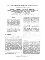
time t, respectively. This structure is shown in Figure 2.1. This representation
S
1
S
2
S
3
S
n 1
S
n
X
1
X
2
X

3
X
n 1
X
n
Figure 2.1: Dependency graph structure for first-order HMMs for sequences.
of a HMM clearly highlights the conditional independence relations within a
HMM. Specifically, the probability of the state at time t depends only on the
state at time t
1. Similarly, the observation generated at time t only depends
on the state of the model at time t. In the POS tagging application, this means
that we are considering the tag y
t
(recall that we are assuming a one-to-one cor-
respondence between states and tags) of each word x
t
to depend only on the
12 Chapter 2. Directed Graphical Models
tag assigned to the previous word y
t 1
, and each word x
t
to depend only on
the current POS tag y
t
. These conditional independence relations, combined
with the probability chain rule, may be used to factorise the joint distribution
over a state sequence s and observation sequence x into the product of a set of
conditional probabilities:
p

s x p s
1
p x
1
s
1
n
∏
t 2
p s
t
s
t 1
p x
t
s
t
(2.6)
2.2.1 Labelling Sequential Data
As stated above, labelling an observation sequence is the task of identifying
the sequence of labels that best accounts for the observation sequence. In other
words, when choosing the most appropriate label sequence for an observation
sequence x we want to choose the label sequence y
that maximises the condi-
tional probability of the label sequence given the observation sequence:
y
argmax
y
p y x (2.7)
However, since the distribution defined by an HMM is a joint distribution

p
x s over observation and state sequences, the most appropriate label se-
quence for any observation sequence is obtained by finding the finding se-
quence of states s
that maximises the conditional probability of the state se-
quence given the observation sequence, which may be calculated from the joint
distribution using Bayes’ rule:
s
argmax
s
p x s
p x
(2.8)
and then reading off the labels y associated with the states in this sequence.
Finding the optimal state sequence is most efficiently performed using a dy-
namic programming technique known as Viterbi alignment. The Viterbi algo-
rithm is described in [45].
2.2. Hidden Markov Models 13
2.2.2 Limitations of Generative Models
Despite their widespread use, HMMs and other generative models are not the
most appropriate sort of model for the task of labelling sequential data. Gen-
erative models define a joint probability distribution p x y over observation
and label sequences. This is useful if the trained model is to be used to gener-
ate data, however, the distribution of interest when labelling data is the condi-
tional distribution p
y x over label sequences given the observation sequence
in question. Defining a joint distribution over label and observation sequences
means that all possible observation sequences must be enumerated – a task
which is hard if observations elements are assumed to have long-distance de-
pendencies. Therefore, generative models must make strict independence as-

sumptions in order to make inference tractable. In the case of an HMM, the
observation at time t is assumed to depend only on the state at time t, ensuring
that each observation element is treated as an isolated unit, independent from
all other elements in the sequence.
In fact, most sequential data cannot be accurately represented as a set of iso-
lated elements. Such data contain long-distance dependencies between ob-
servation elements and benefit from being represented in by a model that al-
lows such dependencies and enables observation sequences to be represented
by non-independent overlapping features. For example, when assigning POS
tags to words, performance is improved significantly by assigning tags on the
basis of complex feature sets that utilise information such as the identity of
the current word, the identity of surrounding words, the previous two POS
tags, whether a word starts with a number or upper case letter, whether the
word contains a hyphen, and the suffix of the word [46, 31]. These features are
not independent (for example, the suffix of the current word is entirely depen-
dent on the identity of the word) and contain dependencies other than those
between the current and previous tags, and the current word and current tag.
Fortunately, the use of conditional models for labelling data sequences pro-
vides a convenient method of overcoming the strong independence assump-
14 Chapter 2. Directed Graphical Models
tions required by practical generative models. Rather than modelling the joint
probability distribution p
x s over observations and states, conditional mod-
els define a conditional distribution p
s x over state sequences given a partic-
ular observation sequence. This means that when identifying the most likely
state sequence for a given observation sequence, the conditional distribution
may be used directly, rather than using
s
argmax

s
p s x argmax
s
p x s
p x
(2.9)
which requires enumeration of all possible observation sequences so that the
marginal probability p
x can be calculated.
2.3 Maximum Entropy Markov Models
Maximum entropy Markov models [33] are a form of conditional model for
labelling sequential data designed to address the problems that arise from the
generative nature and strong independence assumptions of hidden Markov
models. MEMMs have been applied to a number of labelling and segmenta-
tion tasks including POS tagging [31] and the segmentation of text documents
[33].
Like HMMs, MEMMs are also based on the concept of a probabilistic finite
state model, however, rather generating observations the model is a proba-
bilistic finite state acceptor [40] that outputs label sequences when presented
with an observation sequence. MEMMs consider observation sequences to be
events to be conditioned upon rather than generated. Therefore, instead of
defining two types of distribution – a transition distribution P
s s represent-
ing the probability of moving from state s to state s
and an observation dis-
tribution P
x s representing the probability of emitting observation x when in
state s – a MEMM has only a single set of
S separately trained distributions of
the form

P
s
s x P s s x (2.10)
2.3. Maximum Entropy Markov Models 15
which represent the probability of moving from state s to s on observation x.
The fact that each of these functions is specific to a given state means that the
choice of possible states at any given instant in time t
1 depends only on the
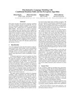
state of the model at time t. The use of state-observation transition functions
which are conditioned on the observations means that the dependency graph
for a MEMM takes the form shown in Figure 2.2. Note that the observation
S
1
S
2
S
3
S
n 1
S
n
X
1
X
2
X
3
X
n 1
X

n
Figure 2.2: Graphical structure of first-order MEMMs for sequences. The variables
corresponding to unshaded nodes are not generated by the model.
sequence is being conditioned upon rather than generated, and so the distri-
bution associated with the graph is the joint distribution of only those random
variables S
t
representing the state of the MEMM at time t. Assuming that each
state corresponds to a particular label, the chain rule of probability and the
conditional independences embodied in the MEMM dependency graph struc-
ture may be used to factorise the joint distribution over label sequences y given
the observation sequence x as:
p
yx p y
1
x
1
n
∏
t 2
p y
t
y
t 1
x
t
(2.11)
Treating observations as events to be conditioned upon rather than generated
means that the probability of each transition may depend on non-independent,
interacting features of the observation sequence. McCallum et al. [33] do this

by making use of the maximum entropy framework, which is discussed in
detail in Chapter 3, and defining each state-observation transition function to