conditional random fields for object recognition

Conditional Random Fields for Object
Recognition
Ariadna Quattoni Michael Collins Trevor Darrell
MIT Computer Science and Artificial Intelligence Laboratory
Cambridge, MA 02139
{ariadna, mcollins, trevor}@csail.mit.edu
Abstract
We present a discriminative part-based approach for the recognition of
object classes from unsegmented cluttered scenes. Objects are modeled
as flexible constellations of parts conditioned on local observations found
by an interest operator. For each object class the probability of a given
assignment of parts to local features is modeled by a Conditional Ran-
dom Field (CRF). We propose an extension of the CRF framework that
incorporates hidden variables and combines class conditional CRFs into
a unified framework for part-based object recognition. The parameters of
the CRF are estimated in a maximum likelihood framework and recogni-
tion proceeds by finding the most likely class under our model. The main
advantage of the proposed CRF framework is that it allows us to relax the
assumption of conditional independence of the observed data (i.e. local
features) often used in generative approaches, an assumption that might
be too restrictive for a considerable number of object classes.
1 Introduction
The problem that we address in this paper is that of learning object categories from super-
vised data. Given a training set of n pairs (x
i
, y
i
), where x
i
is the ith image and y
i

is the
category of the object present in x
i
, we would like to learn a model that maps images to
object categories. In particular, we are interested in learning to recognize rigid objects such
as cars, motorbikes, and faces from one or more fixed view-points.
The part-based models we consider represent images as sets of patches, or local features,
which are detected by an interest operator such as that described in [4]. Thus an image
x
i
can be considered to be a vector {x
i,1
, . . . , x
i,m
} of m patches. Each patch x
i,j
has
a feature-vector representation φ(x
i,j
) ∈ R
d
; the feature vector might capture various
features of the appearance of a patch, as well as features of its relative location and scale.
This scenario presents an interesting challenge to conventional classification approaches in
machine learning, as the input space x
i
is naturally represented as a set of feature-vectors
{φ(x
i,1
), . . . , φ(x

i,m
)} rather than as a single feature vector. Moreover, the local patches
underlying the local feature vectors may have complex interdependencies: for example,
they may correspond to different parts of an object, whose spatial arrangement is important
to the classification task.
The most widely used approach for part-based object recognition is the generative model
proposed in [1]. This classification system models the appearance, spatial relations and
co-occurrence of local parts. One limitation of this framework is that to make the model
computationally tractable one has to assume the independence of the observed data (i.e.,
local features) given their assignment to parts in the model. This assumption might be too
restrictive for a considerable number of object classes made of structured patterns.
A second limitation of generative approaches is that they require a model P (x
i,j
|h
i,j
) of
patches x
i,j
given underlying variables h
i,j
(e.g., h
i,j
may be a hidden variable in the
model, or may simply be y
i
). Accurately specifying such a generative model may be chal-
lenging – in particular in cases where patches overlap one another, or where we wish to
allow a hidden variable h
i,j
to depend on several surrounding patches. A more direct ap-

proach may be to use a feature vector representation of patches, and to use a discriminative
learning approach. We follow an approach of this type in this paper.
Similar observations concerning the limitations of generative models have been made in
the context of natural language processing, in particular in sequence-labeling tasks such as
part-of-speech tagging [7, 5, 3] and in previous work on conditional random fields (CRFs)
for vision [2]. In sequence-labeling problems for NLP each observation x
i,j
is typically
the j’th word for some input sentence, and h
i,j
is a hidden state, for example representing
the part-of-speech of that word. Hidden Markov models (HMMs), a generative approach,
require a model of P (x
i,j
|h
i,j
), and this can be a challenging task when features such as
word prefixes or suffixes are included in the model, or where h
i,j
is required to depend
directly on words other than x
i,j
. This has led to research on discriminative models for se-
quence labeling such as MEMM’s [7, 5] and conditional random fields (CRFs)[3]. A strong
argument for these models as opposed to HMMs concerns their flexibility in terms of rep-
resentation, in that they can incorporate essentially arbitrary feature-vector representations
φ(x
i,j
) of the observed data points.
We propose a new model for object recognition based on Conditional Random Fields. We

model the conditional distribution p(y|x) directly. A key difference of our approach from
previous work on CRFs is that we make use of hidden variables in the model. In previous
work on CRFs (e.g., [2, 3]) each “label” y
i
is a sequence h
i
= {h
i,1
, h
i,2
, . . . , h
i,m
} of
labels h
i,j
for each observation x
i,j
. The label sequences are typically taken to be fully
observed on training examples. In our case the labels y
i
are unstructured labels from some
fixed set of object categories, and the relationship between y
i
and each observation x
i,j
is
not clearly defined. Instead, we model intermediate part-labels h
i,j
as hidden variables in
the model. The model defines conditional probabilities P (y, h | x), and hence indirectly

P (y | x) =

h
P (y, h | x), using a CRF. Dependencies between the hidden variables
h are modeled by an undirected graph over these variables. The result is a model where
inference and parameter estimation can be carried out using standard graphical model al-
gorithms such as belief propagation [6].
2 The Model
2.1 Conditional Random Fields with Hidden Variables
Our task is to learn a mapping from images x to labels y. Each y is a member of a set Y
of possible image labels, for example, Y = {background, car}. We take each image x
to be a vector of m “patches” x = {x
1
, x
2
, . . . , x
m
}.
1
Each patch x
j
is represented by a
feature vector φ(x
j
) ∈ R
d
. For example, in our experiments each x
j
corresponds to a patch
that is detected by the feature detector in [4]; section [3] gives details of the feature-vector

representation φ(x
j
) for each patch. Our training set consists of labeled images (x
i
, y
i
) for
i = 1 . . . n, where each y
i
∈ Y, and each x
i
= {x
i,1
, x
i,2
, . . . , x
i,m
}. For any image x
we also assume a vector of “parts” variables h = {h
1
, h
2
, . . . , h
m
}. These variables are
not observed on training examples, and will therefore form a set of hidden variables in the
1
Note that the number of patches m can vary across images, and did vary in our experiments. For
convenience we use notation where m is fixed across different images; in reality it will vary across
images but this leads to minor changes to the model.

model. Each h
j
is a member of H where H is a finite set of possible parts in the model.
Intuitively, each h
j
corresponds to a labeling of x
j
with some member of H. Given these
definitions of image-labels y, images x, and part-labels h, we will define a conditional
probabilistic model:
P (y, h | x, θ) =
e
Ψ(y, h,x; θ)

y

,h
e
Ψ(y

,h,x;θ)
. (1)
Here θ are the parameters of the model, and Ψ(y, h, x; θ) ∈ R is a potential function
parameterized by θ. We will discuss the choice of Ψ shortly. It follows that
P (y | x, θ) =

h
P (y, h | x, θ) =

h

e
Ψ(y, h, x;θ)

y

,h
e
Ψ(y

,h,x;θ)
. (2)
Given a new test image x, and parameter values θ
∗
induced from a training example, we
will take the label for the image to be arg max
y ∈Y
P (y | x, θ
∗
). Following previous work
on CRFs [2, 3], we use the following objective function in training the parameters:
L(θ) =

i
log P(y
i
| x
i
, θ) −
1
2σ

2
||θ||
2
(3)
The first term in Eq. 3 is the log-likelihood of the data. The second term is the log of a
Gaussian prior with variance σ
2
, i.e., P (θ) ∼ exp

1
2σ
2
||θ||
2

. We will use gradient ascent
to search for the optimal parameter values, θ
∗
= arg max
θ
L(θ), under this criterion.
We now turn to the definition of the potential function Ψ(y, h, x; θ). We assume an undi-
rected graph structure, with the hidden variables {h
1
, . . . , h
m
} corresponding to vertices
in the graph. We use E to denote the set of edges in the graph, and we will write (j, k) ∈ E
to signify that there is an edge in the graph between variables h
j

and h
k
. In this paper we
assume that E is a tree.
2
We define Ψ to take the following form:
Ψ(y, h, x; θ) =
m

j=1

l
f
1
l
(j, y, h
j
, x)θ
1
l
+

(j,k)∈E

l
f
2
l
(j, k, y, h
j

, h
k
, x)θ
2
l
(4)
where f
1
l
, f
2
l
are functions defining the features in themodel, andθ
1
l
, θ
2
l
are the components
of θ. The f
1
features depend on single hidden variable values in the model, the f
2
features
can depend on pairs of values. Note that Ψ is linear in the parameters θ, and the model in
Eq. 1 is a log-linear model. Moreover the features respect the structure of the graph, in that
no feature depends on more than two hidden variables h
j
, h
k

, and if a feature does depend
on variables h
j
and h
k
there must be an edge (j, k) in the graph E.
Assuming that the edges in E form a tree, and that Ψ takes the form in Eq. 4, then exact
methods exist for inference and parameter estimation in the model. This follows because
belief propagation [6] can be used to calculate the following quantities in O(|E||Y|) time:
∀y ∈ Y, Z(y | x, θ) =

h
exp{Ψ(y, h, x; θ)}
∀y ∈ Y, j ∈ 1 . . . m, a ∈ H, P (h
j
= a | y, x, θ) =

h:h
j
=a
P (h | y, x, θ)
∀y ∈ Y, (j, k) ∈ E, a, b ∈ H, P (h
j
= a, h
k
= b | y, x, θ) =

h:h
j
=a,h

k
=b
P (h | y, x, θ)
2
This will allow exact methods for inference and parameter estimation in the model, for example
using belief propagation. If E contains cycles then approximate methods, such as loopy belief-
propagation, may be necessary for inference and parameter estimation.
The first term Z(y | x, θ) is a partition function defined by a summation over
the h variables. Terms of this form can be used to calculate P(y | x, θ) =
Z(y | x, θ)/

y

Z(y

| x, θ). Hence inference—calculation of arg max P (y | x, θ)—
can be performed efficiently in the model. The second and third terms are marginal distri-
butions over individual variables h
j
or pairs of variables h
j
, h
k
corresponding to edges in
the graph. The next section shows that the gradient of L(θ) can be defined in terms of these
marginals, and hence can be calculated efficiently.
2.2 Parameter Estimation Using Belief Propagation
This section considers estimation of the parameters θ
∗
= arg max L(θ) from a training

sample, where L(θ) is defined in Eq. 3. In our work we used a conjugate-gradient method
to optimize L(θ) (note that due to the use of hidden variables, L(θ) has multiple local
minima, and our method is therefore not guaranteed to reach the globally optimal point).
In this section we describe how the gradient of L(θ) can be calculated efficiently. Consider
the likelihood term that is contributed by the i’th training example, defined as:
L
i
(θ) = log P(y
i
| x
i
, θ) = log


h
e
Ψ(y
i
,h,x
i
;θ)

y

,h
e
Ψ(y

,h,x
i

;θ)
.

(5)
We first consider derivatives with respect to the parameters θ
1
l
corresponding to features
f
1
l
(j, y, h
j
, x) that depend on single hidden variables. Taking derivatives gives
∂L
i
(θ)
∂θ
1
l
=

h
P (h | y
i
, x
i
, θ)
∂Ψ(y
i

, h, x
i
; θ)
∂θ
1
l
−

y

,h
P (y

, h | x
i
, θ)
∂Ψ(y

, h, x
i
; θ)
∂θ
1
l
=

h
P (h | y
i
, x

i
, θ)
m

j=1
f
1
l
(j, y
i
, h
j
, x
i
) −

y

,h
P (y

, h | x
i
, θ)
m

j=1
f
1
l

(j, y

, h
j
, x
i
)
=

j,a
P (h
j
= a | y
i
, x
i
, θ)f
1
l
(j, y
i
, a, x
i
) −

y

,j,a
P (h
j

= a, y

| x
i
, θ)f
1
l
(j, y

, a, x
i
)
It follows that
∂L
i
(θ)
∂θ
1
l
can be expressed in terms of components P (h
j
= a | x
i
, θ) and
P (y | x
i
, θ), which can be calculated using belief propagation, provided that the graph E
forms a tree structure. A similar calculation gives
∂L
i

(θ )
∂θ
2
l
=

(j,k)∈E,a,b
P (h
j
= a, h
k
= b | y
i
, x
i
, θ)f
2
l
(j, k, y
i
, a, b, x
i
)
−

y

,(j,k)∈E,a,b
P (h
j

= a, h
k
= b, y

| x
i
, θ)f
2
l
(j, k, y

, a, b, x
i
)
hence ∂L
i
(θ)/∂θ
2
l
can also be expressed in terms of expressions that can be calculated
using belief propagation.
2.3 The Specific Form of our Model
We now turn to the specific form for the model in this paper. We define
Ψ(y, h, x; θ) =

j
φ(x
j
) · θ(h
j

) +

j
θ(y, h
j
) +

(j,k)∈E
θ(y, h
j
, h
k
) (6)
Here θ(k) ∈ R
d
for k ∈ H is a parameter vector corresponding to the k’th part label. The
inner-product φ(x
j
) · θ(h
j
) can be interpreted as a measure of the compatibility between
patch x
j
and part-label h
j
. Each parameter θ(y, k) ∈ R for k ∈ H, y ∈ Y can be
interpreted as a measure of the compatibility between part k and label y. Finally, each
parameter θ(y, k, l) ∈ R for y ∈ Y, and k, l ∈ H measures the compatibility between an
edge with labels k and l and the label y. It is straightforward to verify that the definition in
Eq. 6 can be written in the same form as Eq. 4. Hence belief propagation can be used for

inference and parameter estimation in the model.
The patches x
i,j
in each image are obtained using the SIFT detector [4]. Each patch x
i,j
is then represented by a feature vector φ(x
i,j
) that incorporates a combination of SIFT and
relative location and scale features.
The tree E is formed by running a minimum spanning tree algorithm over the parts h
i,j
,
where the cost of an edge in the graph between h
i,j
and h
i,k
is taken to be the distance
between x
i,j
and x
i,k
in the image. Note that the structure of E will vary across different
images. Our choice of E encodes our assumption that parts conditioned on features that are
spatially close are more likely to be dependent. In the future we plan to experiment with
the minimum spanning tree approach under other definitions of edge-cost. We also plan to
investigate more complex graph structures that involve cycles, which may require approx-
imate methods such as loopy belief propagation for parameter estimation and inference.
3 Experiments
We carried out three sets of experiments on a number of different data sets.
3

The first
two experiments consisted of training a two class model (object vs. background) to distin-
guish between a category from a single viewpoint and background. The third experiment
consisted of training a multi-class model to distinguish between n classes.
The only parameter that was adjusted in the experiments was the scale of the images upon
which the interest point detector was run. In particular, we adjusted the scale on the car
side data set: in this data set the images were too small and without this adjustment the
detector would fail to find a significant amount of features.
For the experiments we randomly split each data set into three separate data sets: training,
validation and testing. We use the validation data set to set the variance parameters σ
2
of
the gaussian prior.
3.1 Results
In figure 2.a we show how the number of parts in the model affects performance. In the case
of the car side data set, the ten-part model shows a significant improvement compared to
the five parts model while for the car rear data set the performance improvement obtained
by increasing the number of parts is not as significant. Figure 2.b shows a performance
comparison with previous approaches [1] tested on the same data set (though on a different
partition). We observe an improvement between 2 % and 5 % for all data sets.
Figures 3 and 4 show results for the multi-class experiments. Notice that random perfor-
mance for the animal data set would be 25 % across the diagonal. The model exhibits
best performance for the Leopard data set, for which the presence of part 1 alone is a clear
predictor of the class. This shows again that our model can learn discriminative part distri-
butions for each class. Figure 3 shows results for a multi-view experiment where the task
is two distinguish between two different views of a car and background.
3
The images were obtained from and the
car side images from cogcomp/Data/Car/. Notice, that since our algorithm
does not currently allow for the recognition of multiple instances of an object we test it on a partition

of the the training set in cogcomp/Data/Car/ and not on the testing set in that
site. The animals data set is a subset of Caltech’s 101 categories data set.
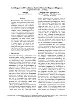
Figure 1: Examples of the most likely assignment of parts to features for the two class
experiments (car data set).
(a)
Data set 5 parts 10 parts
Car Side 94 % 99 %
Car Rear 91 % 91.7 %
(b)
Data set Our Model Others [1]
Car Side 99 % -
Car Rear 94.6 % 90.3 %
Face 99 % 96.4 %
Plane 96 % 90.2 %
Motorbike 95 % 92.5 %
Figure 2: (a) Equal Error Rates for the car side and car rear experiments with different
number of parts. (b) Comparative Equal Error Rates.
Figure 1 displays the Viterbi labeling
4
for a set of example images showing the most likely
assignment of local features to parts in the model. Figure 6 shows the mean and variance
of each part’s location for car side images and background images. The mean and variance
of each part’s location for the car side images were calculated in the following manner:
First we find for every image classified as class a the most likely part assignment under our
model. Second, we calculate the mean and variance of positions of all local features that
were assigned to the same part. Similarly Figure 5 shows part counts among the Viterbi
paths assigned to examples of a given class.
As can be seen in Figure 6 , while the mean location of a given part in the background
images and the mean location of the same part in the car images are very similar, the parts
in the car have a much tighter distribution which seems to suggest that the model is learning

the shape of the object.
As shown in Figure 5 the model has also learnt discriminative part distributions for each
class, for example the presence of part 1 seems to be a clear predictor for the car class. In
general part assignments seem to rely on a combination of appearance and relative location.
Part 1, for example, is assigned to wheel like patterns located on the left of the object.
4
This is the labeling h
∗
= arg max
h
P (h | y, x, θ) where x is an image and y is the label for
the image under the model.
Data set Precision Recall
Car Side 87.5 % 98 %
Car Rear 87.4 % 86.5 %
Figure 3: Precision and recall results for 3 class experiment.
Data set Leopards Llamas Rhinos Pigeons
Leopards 91 % 2 % 0 % 7 %
Llamas 0 % 50 % 27 % 23 %
Rhinos 0 % 40 % 46 % 14 %
Pigeons 0 % 30 % 20 % 50 %
Figure 4: Confusion table for 4 class experiment.
However, the parts might not carry semantic meaning. It appears that the model has learnt
a vocabulary of very general parts with significant variability in appearance and learns to
discriminate between classes by capturing the most likely arrangement of these parts for
each class.
In some cases the model relies more heavily on relative location than appearance because
the appearance information might not be very useful for discriminating between the two
classes. One of the reasons for this is that the detector produces a large number of false de-
tections, making the appearance data too noisy for discrimination. The fact that the model

is able to cope with this lack of discriminating appearance information illustrates its flexible
data-driven nature. This can be a desirable model property of a general object recognition
system, because for some object classes appearance is the important discriminant (i.e., in
textured classes) while for others shape may be important (i.e., in geometrically constrained
classes).
One noticeable difference between our model and similar part-based models is that our
model learns large parts composed of small local features. This is not surprising given how
the part dependencies were built (i.e., through their position in minimum spanning tree):
the potential functions defined on pairs of hidden variables tend to smooth the allocation of
parts to patches.
3
8
4
5
1
3
4
5
6
7
8
Figure 5: Graph showing part counts for the background (left) and car side images (right)
4 Conclusions and Further Work
In this work we have presented a novel approach that extends the CRF framework by in-
corporating hidden variables and combining class conditional CRFs into an unified frame-
work for object recognition. Similarly to CRFs and other maximum entropy models our
approach allows us to combine arbitrary observation features for training discriminative
classifiers with hidden variables. Furthermore, by making some assumptions about the
joint distribution of hidden variables one can derive efficient training algorithms based on
dynamic programming.

−200 −150 −100 −50 0 50 100 150 200
−200
−150
−100
−50
0
50
100
150
200
Background Shape
5
3
4
8
−200 −150 −100 −50 0 50 100 150 200
−200
−150
−100
−50
0
50
100
150
200
Car Shape
5
3
1
9

7
6
4
8
(a) (b)
Figure 6: (a) Graph showing mean and variance of locations for the different parts for the
car side images; (b) Mean and variance of part locations for the background images.
The main limitation of our model is that it is dependent on the feature detector picking up
discriminative features of the object. Furthermore, our model might learn to discriminate
between classes based on the statistics of the feature detector and not the true underlying
data, to which it has no access. This is not a desirable property since it assumes the feature
detector to be consistent. As future work we would like to incorporate the feature detection
process into the model.
References
[1] R. Fergus, P. Perona,and A. Zisserman. Object class recognition by unsupervised scale-invariant
learning. In Proceedings of the IEEE Conference on Computer Vision and Pattern Recogni-
tion,volume 2, pages 264-271, June 2003.
[2] S. Kumar and M. Hebert. Discriminative random fields: A framework for contextual interaction
in classification. In IEEE Int Conference on Computer Vision,volume 2, pages 1150-1157, June
2003.
[3] J. Lafferty,A. McCallum and F. Pereira. Conditional random fields: Probabilistic models for
segmenting and labeling sequence data. In Proc. Int Conf. on Machine Learning, 2001.
[4] D. Lowe. Object Recognition from local scale-invariant features. In IEEE Int Conference on
Computer Vision, 1999.
[5] A. McCallum, D. Freitag, and F. Pereira. Maximum entropy markov models for information
extraction and segmentation. In ICML-2000, 2000.
[6] J. Pearl. Probabilistic Reasoning in Intelligent Systems: Networks of Plausible Inference. Mor-
gan Kaufmann,1988.
[7] A. Ratnaparkhi. A maximum entropy part-of-speech tagger. In EMNLP, 1996.