- Trang chủ >>
- Khoa Học Tự Nhiên >>
- Vật lý
mase, mase. continuum mechanics for engineers (crc, 1999)(380s)
Bạn đang xem bản rút gọn của tài liệu. Xem và tải ngay bản đầy đủ của tài liệu tại đây (4.6 MB, 380 trang )
CONTINUUM
MECHANICS
for ENGINEERS
Second Edition
© 1999 by CRC Press LLC
G. Thomas Mase
George E. Mase
CONTINUUM
MECHANICS
for ENGINEERS
Second Edition
Boca Raton London New York Washington, D.C.
CRC Press
Library of Congress Cataloging-in-Publication Data
Mase, George Thomas.
Continuum mechanics for engineers / G. T. Mase and G. E. Mase.
2nd ed.
p. cm.
Includes bibliographical references (p. )and index.
ISBN 0-8493-1855-6 (alk. paper)
1. Continuum mechanics. I. Mase, George E.
QA808.2.M364 1999
531—dc21
99-14604
CIP
This book contains information obtained from authentic and highly regarded sources.
Reprinted material is quoted with permission, and sources are indicated. A wide variety of
references are listed. Reasonable efforts have been made to publish reliable data and informa-
tion, but the author and the publisher cannot assume responsibility for the validity of all
materials or for the consequences of their use.
Neither this book nor any part may be reproduced or transmitted in any form or by any
means, electronic or mechanical, including photocopying, microfilming, and recording, or by
any information storage or retrieval system, without prior permission in writing from the
publisher.
The consent of CRC Press LLC does not extend to copying for general distribution, for
promotion, for creating new works, or for resale. Specific permission must be obtained in writing
from CRC Press LLC for such copying.
Direct all inquiries to CRC Press LLC, 2000 N.W. Corporate Blvd., Boca Raton, Florida 33431.
Trademark Notice:
Product or corporate names may be trademarks or registered trademarks,
and are only used for identification and explanation, without intent to infringe.
© 1999 by CRC Press LLC
No claim to original U.S. Government works
International Standard Book Number 0-8493-1855-6
Library of Congress Card Number 99-14604
Printed in the United States of America 1 2 3 4 5 6 7 8 9 0
Printed on acid-free paper
Preface to Second Edition
It is fitting to start this, the preface to our second edition, by thanking all of
those who used the text over the last six years. Thanks also to those of you
who have inquired about this revised and expanded version. We hope that
you find this edition as helpful as the first to introduce seniors or graduate
students to continuum mechanics.
The second edition, like its predecessor, is an outgrowth of teaching con-
tinuum mechanics to first- or second-year graduate students. Since my father
is now fully retired, the course is being taught to students whose final degree
will most likely be a Masters at Kettering University. A substantial percent-
age of these students are working in industry, or have worked in industry,
when they take this class. Because of this, the course has to provide the stu-
dents with the fundamentals of continuum mechanics and demonstrate its
applications.
Very often, students are interested in using sophisticated simulation pro-
grams that use nonlinear kinematics and a variety of constitutive relation-
ships. Additions to the second edition have been made with these needs in
mind. A student who masters its contents should have the mechanics foun-
dation necessary to be a skilled user of today’s advanced design tools such as
nonlinear, explicit finite elements. Of course, students need to augment the
mechanics foundation provided herein with rigorous finite element training.
Major highlights of the second edition include two new chapters, as well as
significant expansion of two other chapters. First, Chapter Five,
Fundamental Laws and Equations, was expanded to add material regarding
constitutive equation development. This includes material on the second law
of thermodynamics and invariance with respect to restrictions on constitu-
tive equations. The first edition applications chapter covering elasticity and
fluids has been split into two separate chapters. Elasticity coverage has been
expanded by adding sections on Airy stress functions, torsion of noncircular
cross sections, and three-dimensional solutions. A chapter on nonlinear
elasticity has been added to give students a molecular and phenomenological
introduction to rubber-like materials. Finally, a chapter introducing students
to linear viscoelasticity is given since many important modern polymer
applications involve some sort of rate dependent material response.
It is not easy singling out certain people in order to acknowledge their help
while not citing others; however, a few individuals should be thanked.
Ms. Sheri Burton was instrumental in preparation of the second edition
manuscript. We wish to acknowledge the many useful suggestions by users of
the previous edition, especially Prof. Morteza M. Mehrabadi, Tulane University,
for his detailed comments. Thanks also go to Prof. Charles Davis, Kettering
© 2001 by CRC Press LLC
© 1999 by CRC Press LLC
University, for helpful comments on the molecular approach to rubber and
thermoplastic elastomers. Finally, our families deserve sincerest thanks for
their encouragement.
It has been a great thrill to be able to work as a father-son team in publish-
ing this text, so again we thank you, the reader, for your interest.
G. Thomas Mase
Flint, Michigan
George E. Mase
East Lansing, Michigan
© 2001 by CRC Press LLC
© 1999 by CRC Press LLC
Preface to the First Edition
(Note: Some chapter reference information has changed in the Second Edition.)
Continuum mechanics is the fundamental basis upon which several graduate
courses in engineering science such as elasticity, plasticity, viscoelasticity, and
fluid mechanics are founded. With that in mind, this introductory treatment
of the principles of continuum mechanics is written as a text suitable for a
first course that provides the student with the necessary background in con-
tinuum theory to pursue a formal course in any of the aforementioned sub-
jects. We believe that first-year graduate students, or upper-level
undergraduates, in engineering or applied mathematics with a working
knowledge of calculus and vector analysis, and a reasonable competency in
elementary mechanics will be attracted to such a course.
This text evolved from the course notes of an introductory graduate contin-
uum mechanics course at Michigan State University, which was taught on a
quarter basis. We feel that this text is well suited for either a quarter or semes-
ter course in continuum mechanics. Under a semester system, more time can
be devoted to later chapters dealing with elasticity and fluid mechanics. For
either a quarter or a semester system, the text is intended to be used in con-
junction with a lecture course.
The mathematics employed in developing the continuum concepts in the
text is the algebra and calculus of Cartesian tensors; these are introduced and
discussed in some detail in Chapter Two, along with a review of matrix meth-
ods, which are useful for computational purposes in problem solving.
Because of the introductory nature of the text, curvilinear coordinates are not
introduced and so no effort has been made to involve general tensors in this
work. There are several books listed in the Reference Section that a student
may refer to for a discussion of continuum mechanics in terms of general ten-
sors. Both indicial and symbolic notations are used in deriving the various
equations and formulae of importance.
Aside from the essential mathematics presented in Chapter Two, the book
can be seen as divided into two parts. The first part develops the principles
of stress, strain, and motion in Chapters Three and Four, followed by the der-
ivation of the fundamental physical laws relating to continuity, energy, and
momentum in Chapter Five. The second portion, Chapter Six, presents some
elementary applications of continuum mechanics to linear elasticity and clas-
sical fluids behavior. Since this text is meant to be a first text in continuum
mechanics, these topics are presented as constitutive models without any dis-
cussion as to the theory of how the specific constitutive equation was
derived. Interested readers should pursue more advanced texts listed in the
© 2001 by CRC Press LLC
© 1999 by CRC Press LLC
Reference Section for constitutive equation development. At the end of each
chapter (with the exception of Chapter One) there appears a collection of
problems, with answers to most, by which the student may reinforce her/his
understanding of the material presented in the text. In all, 186 such practice
problems are provided, along with numerous worked examples in the text
itself.
Like most authors, we are indebted to many people who have assisted in
the preparation of this book. Although we are unable to cite each of them
individually, we are pleased to acknowledge the contributions of all. In addi-
tion, sincere thanks must go to the students who have given feedback from
the classroom notes which served as the forerunner to the book. Finally, and
most sincerely of all, we express special thanks to our family for their encour-
agement from beginning to end of this work.
G. Thomas Mase
Flint, Michigan
George E. Mase
East Lansing, Michigan
© 2001 by CRC Press LLC
© 1999 by CRC Press LLC
Authors
G. Thomas Mase
, Ph.D. is Associate Professor of Mechanical Engineering at
Kettering University (formerly GMI Engineering & Management Institute),
Flint, Michigan. Dr. Mase received his B.S. degree from Michigan State Uni-
versity in 1980 from the Department of Metallurgy, Mechanics, and Materials
Science. He obtained his M.S. and Ph.D. degrees in 1982 and 1985, respec-
tively, from the Department of Mechanical Engineering at the University of
California, Berkeley. Immediately after receiving his Ph.D., he worked for
two years as a senior research engineer in the Engineering Mechanics Depart-
ment at General Motors Research Laboratories. In 1987, he accepted an assis-
tant professorship at the University of Wyoming and subsequently moved to
Kettering University in 1990. Dr. Mase is a member of numerous professional
societies including the American Society of Mechanical Engineers, Society of
Automotive Engineers, American Society of Engineering Education, Society
of Experimental Mechanics, Pi Tau Sigma, Sigma Xi, and others. He received
an ASEE/NASA Summer Faculty Fellowship in 1990 and 1991 to work at
NASA Lewis Research Center. While at the University of California, he twice
received a distinguished teaching assistant award in the Department of
Mechanical Engineering. His research interests include design with explicit
finite element simulation. Specific areas include golf equipment design and
vehicle crashworthiness.
George E. Mase
, Ph.D., is Emeritus Professor, Department of Metallurgy,
Mechanics, and Materials Science (MMM), College of Engineering, at Michi-
gan State University. Dr. Mase received a B.M.E. in Mechanical Engineering
(1948) from the Ohio State University, Columbus. He completed his Ph.D. in
Mechanics at Virginia Polytechnic Institute and State University (VPI),
Blacksburg, Virginia (1958). Previous to his initial appointment as Assistant
Professor in the Department of Applied Mechanics at Michigan State Univer-
sity in 1955, Dr. Mase taught at Pennsylvania State University (instructor),
1950 to 1951, and at Washington University, St. Louis, Missouri (assistant pro-
fessor), 1951 to 1954. He was appointed associate professor at Michigan State
University in 1959 and professor in 1965, and served as acting chairperson of
the MMM Department, 1965 to 1966 and again in 1978 to 1979. He taught as
visiting assistant professor at VPI during the summer terms, 1953 through
1956. Dr. Mase holds membership in Tau Beta Pi and Sigma Xi. His research
interests and publications are in the areas of continuum mechanics, viscoelas-
ticity, and biomechanics.
© 2001 by CRC Press LLC
© 1999 by CRC Press LLC
Nomenclature
x
1
, x
2
, x
3
or
x
i
or
x
Rectangular Cartesian coordinates
x
1
*
,
x
2
*
,
x
3
*
Principal stress axes
Unit vectors along coordinate axes
Kronecker delta
Permutation symbol
Partial derivative with respect to time
Spatial gradient operator
١
φ
=
grad
φ
=
φ
,j
Scalar gradient
١
v =
∂
j
v
i
=
v
i,j
Vector gradient
∂
j
v
j
=
v
j
,
j
Divergence of vector
v
ε
ijk
v
k
,
j
Curl of vector
v
b
i
or
b
Body force (force per unit mass)
p
i
or
p
Body force (force per unit volume)
f
i
or
f
Surface force (force per unit area)
V
Total volume
V
.o
Referential total volume
∆
V
Small element of volume
dV
Infinitesimal element of volume
S
Total surface
S
o
Referential total surface
∆
S
Small element of surface
dS
Infinitesimal element of surface
ρ
Density
n
i
or Unit normal in the current configuration
N
A
or Unit normal in the reference configuration
Traction vector
ˆ
,
ˆ
,
ˆ
ee e
123
δ
ij
ε
ijk
∂
t
∂
x
ˆ
n
ˆ
N
t
i
ˆˆ
nn
t
() ()
or
© 2001 by CRC Press LLC
© 1999 by CRC Press LLC
σ
N
Normal component of traction vector
σ
S
Shear component of traction vector
σ
ij
Cauchy stress tensor’s components
Cauchy stress components referred to principal axes
Piola-Kirchhoff stress vector referred to referential area
P
iA
First Piola-Kirchhoff stress components
s
AB
Second Piola-Kirchhoff stress components
Principal stress values
I
σ
,
II
σ
,
III
σ
First, second, and third stress invariants
σ
M
=
σ
ii
/3 Mean normal stress
S
ij
Deviatoric stress tensor’s components
I
S
= 0,
II
S
,
III
S
Deviator stress invariants
σ
oct
Octahedral shear stress
a
ij
Transformation matrix
X
I
or
X
Material, or referential coordinates
v
i
or
v
Velocity vector
a
i
or
a
Acceleration components, acceleration vector
u
i
or
u
Displacement components, or displacement vector
d/dt
=
∂/∂
t
+
v
k
∂/∂
x
k
Material derivative operator
F
iA
or
F
Deformation gradient tensor
C
AB
or
C
Green’s deformation tensor
E
AB
or
E
Lagrangian finite strain tensor
c
ij
or
c
Cauchy deformation tensor
e
ij
or
e
Eulerian finite strain tensor
ε
ij
or
ε
Infinitesimal strain tensor
Principal strain values
I
ε
,
II
ε
,
III
ε
Invariants of the infinitesimal strain tensor
B
ij
=
F
iA
F
jA
Components of left deformation tensor
I
1
,
I
2
,
I
3
Invariants of left deformation tensor
σ
ij
*
p
i
o
ˆ
N
()
σσσ
σσ σ
123
() () ()
,,
,,or
I II III
εεε
εε ε
123
() () ()
,,
,,or
I II III
© 2001 by CRC Press LLC
© 1999 by CRC Press LLC
W
Strain energy per unit volume, or strain energy density
Normal strain in the direction
γ
ij
Engineering shear strain
e
=
∆
V/V
=
ε
ii
=
I
ε
Cubical dilatation
η
ij
or
Deviator strain tensor
ω
ij
or
Infinitesimal rotation tensor
ω
j
or
Rotation vector
Stretch ratio, or stretch in the direction on
Stretch ratio in the direction on
ˆ
n
R
ij
or R Rotation tensor
U
AB
or U Right stretch tensor
V
AB
or V Left stretch tensor
L
ij
=
∂
v
i
/
∂
x
j
Spatial velocity gradient
D
ij
Rate of deformation tensor
W
ij
Vorticity, or spin tensor
J = det F Jacobian
P
i
Linear momentum vector
K(t) Kinetic energy
P(t) Mechanical power, or rate of work done by forces
S(t) Stress work
Q Heat input rate
r Heat supply per unit mass
q
i
Heat flux vector
θ
Temperature
g
i
=
θ
,
i
Temperature gradient
u Specific internal energy
η
Specific entropy
ψ
Gibbs free energy
ζ
Free enthalpy
χ
Enthalpy
γ
Specific entropy production
e
ˆ
N
()
ˆ
N
Λ
ˆ
N
()
= dx dX
ˆ
N
λ
ˆ
n
()
= dX dx
© 2001 by CRC Press LLC
© 1999 by CRC Press LLC
Contents
1 Continuum Theory
1.1 The Continuum Concept
1.2 Continuum Mechanics
2 Essential Mathematics
2.1 Scalars, Vectors, and Cartesian Tensors
2.2 Tensor Algebra in Symbolic Notation —
Summation Convention
2.3 Indicial Notation
2.4 Matrices and Determinants
2.5 Transformations of Cartesian Tensors
2.6 Principal Values and Principal Directions of Symmetric
Second-Order Tensors
2.7 Tensor Fields, Tensor Calculus
2.8 Integral Theorems of Gauss and Stokes
Problems
3 Stress Principles
3.1 Body and Surface Forces, Mass Density
3.2 Cauchy Stress Principle
3.3 The Stress Tensor
3.4 Force and Moment Equilibrium, Stress
Tensor Symmetry
3.5 Stress Transformation Laws
3.6 Principal Stresses, Principal Stress Directions
3.7 Maximum and Minimum Stress Values
3.8 Mohr’s Circles for Stress
3.9 Plane Stress
3.10 Deviator and Spherical Stress States
3.11 Octahedral Shear Stress
Problems
4 Kinematics of Deformation and Motion
4.1 Particles, Configurations, Deformation, and Motion
4.2 Material and Spatial Coordinates
4.3 Lagrangian and Eulerian Descriptions
4.4 The Displacement Field
© 2001 by CRC Press LLC
© 1999 by CRC Press LLC
4.5 The Material Derivative
4.6 Deformation Gradients, Finite Strain Tensors
4.7 Infinitesimal Deformation Theory
4.8 Stretch Ratios
4.9 Rotation Tensor, Stretch Tensors
4.10 Velocity Gradient, Rate of Deformation, Vorticity
4.11 Material Derivative of Line Elements, Areas, Volumes
Problems
5 Fundamental Laws and Equations
5.1 Balance Laws, Field Equations, Constitutive
Equations
5.2 Material Derivatives of Line, Surface, and
Volume Integrals
5.3 Conservation of Mass, Continuity Equation
5.4 Linear Momentum Principle, Equations of Motion
5.5 The Piola-Kirchhoff Stress Tensors,
Lagrangian Equations of Motion
5.6 Moment of Momentum (Angular Momentum)
Principle
5.7 Law of Conservation of Energy, The Energy Equation
5.8 Entropy and the Clausius-Duhem Equation
5.9 Restrictions on Elastic Materials by the Second
Law of Thermodynamics
5.10 Invariance
5.11 Restrictions on Constitutive Equations
from Invariance
5.12 Constitutive Equations
References
Problems
6 Linear Elasticity
6.1 Elasticity, Hooke’s Law, Strain Energy
6.2 Hooke’s Law for Isotropic Media, Elastic Constants
6.3 Elastic Symmetry; Hooke’s Law for Anisotropic Media
6.4 Isotropic Elastostatics and Elastodynamics,
Superposition Principle
6.5 Plane Elasticity
6.6 Linear Thermoelasticity
6.7 Airy Stress Function
6.8 Torsion
6.9 Three-Dimensional Elasticity
Problems
© 2001 by CRC Press LLC
© 1999 by CRC Press LLC
7 Classical Fluids
7.1 Viscous Stress Tensor, Stokesian, and
Newtonian Fluids
7.2 Basic Equations of Viscous Flow, Navier-Stokes
Equations
7.3 Specialized Fluids
7.4 Steady Flow, Irrotational Flow, Potential Flow
7.5 The Bernoulli Equation, Kelvin’s Theorem
Problems
8 Nonlinear Elasticity
8.1 Molecular Approach to Rubber Elasticity
8.2 A Strain Energy Theory for Nonlinear Elasticty
8.3 Specific Forms of the Strain Energy
8.4 Exact Solution for an Incompressible, Neo-Hookean
Material
References
Problems
9 Linear Viscoelasticity
9.1 Introduction
9.2 Viscoelastic Constitutive Equations in Linear
Differential Operator Form
9.3 One-Dimensional Theory, Mechanical Models
9.4 Creep and Relaxation
9.5 Superposition Principle, Hereditary Integrals
9.6 Harmonic Loadings, Complex Modulus, and
Complex Compliance
9.7 Three-Dimensional Problems,
The Correspondence Principle
References
Problems
© 2001 by CRC Press LLC
© 1999 by CRC Press LLC
1
Continuum Theory
1.1 The Continuum Concept
The atomic/molecular composition of matter is well established. On a small
enough scale, for instance, a body of aluminum is really a collection of
discrete aluminum atoms stacked on one another in a particular repetitive
lattice. On an even smaller scale, the atoms consist of a core of protons and
neutrons around which electrons orbit. Thus, matter is not continuous. At
the same time, the physical space in which we live is truly a continuum, for
mathematics teaches us that between any two points in space we can always
find another point, regardless of how close together we choose the original
pair. Clearly then, although we may speak of a material body as “occupying”
a region of physical space, it is evident that the body does not totally “fill”
the space it occupies. However, if we accept the continuum concept of matter,
we agree to ignore the discrete composition of material bodies, and to assume
that the substance of such bodies is distributed uniformly throughout, and
completely fills the space it occupies. In keeping with this continuum
model, we assert that matter may be divided indefinitely into smaller and
smaller portions, each of which retains all of the physical properties of the
parent body. Accordingly, we are able to ascribe field quantities such as
density and velocity to each and every point of the region of space which
the body occupies.
The continuum model for material bodies is important to engineers for
two very good reasons. On the scale by which we consider bodies of steel,
aluminum, concrete, etc., the characteristic dimensions are extremely large
compared to molecular distances so that the continuum model provides a
very useful and reliable representation. Additionally, our knowledge of the
mechanical behavior of materials is based almost entirely upon experimental
data gathered by tests on relatively large specimens.
© 1999 by CRC Press LLC
1.2 Continuum Mechanics
The analysis of the kinematic and mechanical behavior of materials modeled
on the continuum assumption is what we know as
continuum mechanics
.
There are two main themes into which the topics of continuum mechanics
are divided. In the first, emphasis is on the derivation of fundamental equa-
tions which are valid for all continuous media. These equations are based
upon universal laws of physics such as the conservation of mass, the prin-
ciples of energy and momentum, etc. In the second, the focus of attention is
on the development of so-called
constitutive equations
characterizing the
behavior of specific idealized materials, the perfectly elastic solid and the
viscous fluid being the best known examples. These equations provide the
focal points around which studies in elasticity, plasticity, viscoelasticity, and
fluid mechanics proceed.
Mathematically, the fundamental equations of continuum mechanics men-
tioned above may be developed in two separate but essentially equivalent
formulations. One, the integral or global form, derives from a consideration
of the basic principles being applied to a finite volume of the material. The
other, a differential or field approach, leads to equations resulting from the
basic principles being applied to a very small (infinitesimal) element of
volume. In practice, it is often useful and convenient to deduce the field
equations from their global counterparts.
As a result of the continuum assumption, field quantities such as density
and velocity which reflect the mechanical or kinematic properties of contin-
uum bodies are expressed mathematically as continuous functions, or at
worst as piecewise continuous functions, of the space and time variables.
Moreover, the derivatives of such functions, if they enter into the theory at
all, likewise will be continuous.
Inasmuch as this is an introductory textbook, we shall make two further
assumptions on the materials we discuss in addition to the principal one of
continuity. First, we require the materials to be
homogeneous,
that is, to have
identical properties at all locations. And second, that the materials be
isotropic
with respect to certain mechanical properties, meaning that those properties
are the same in all directions at a given point. Later, we will relax this isotropy
restriction to discuss briefly anisotropic materials which have important
meaning in the study of composite materials.
© 1999 by CRC Press LLC
2
Essential Mathematics
2.1 Scalars, Vectors, and Cartesian Tensors
Learning a discipline’s language is the first step a student takes towards
becoming competent in that discipline. The language of continuum mechan-
ics is the algebra and calculus of
tensors
. Here, tensors is the generic name
for those mathematical entities which are used to represent the important
physical quantities of continuum mechanics. Only that category of tensors
known as
Cartesian tensors
is used in this text, and definitions of these will
be given in the pages that follow. The tensor equations used to develop the
fundamental theory of continuum mechanics may be written in either of two
distinct notations: the
symbolic notation,
or the
indicial notation.
We shall make
use of both notations, employing whichever is more convenient for the
derivation or analysis at hand, but taking care to establish the interrelation-
ships between the two. However, an effort to emphasize indicial notation in
most of the text has been made. This is because an introductory course must
teach indicial notation to students who may have little prior exposure to the
topic.
As it happens, a considerable variety of physical and geometrical quanti-
ties have important roles in continuum mechanics, and fortunately, each of
these may be represented by some form of tensor. For example, such quan-
tities as
density
and
temperature
may be specified completely by giving their
magnitude, i.e., by stating a numerical value. These quantities are repre-
sented mathematically by
scalars,
which are referred to as
zeroth-order tensors.
It should be emphasized that scalars are not constants, but may actually be
functions of position and/or time. Also, the exact numerical value of a scalar
will depend upon the units in which it is expressed. Thus, the temperature
may be given by either 68°F or 20°C at a certain location. As a general rule,
lowercase Greek letters in italic print such as
α
,
β
,
λ
, etc. will be used as
symbols for scalars in both the indicial and symbolic notations.
Several physical quantities of mechanics such as
force
and
velocity
require
not only an assignment of magnitude, but also a specification of direction
for their complete characterization. As a trivial example, a 20-Newton force
acting vertically at a point is substantially different than a 20-Newton force
© 1999 by CRC Press LLC
acting horizontally at the point. Quantities possessing such directional prop-
erties are represented by
vectors,
which are
first-order tensors.
Geometrically,
vectors are generally displayed as
arrows,
having a definite length (the mag-
nitude), a specified orientation (the direction), and also a sense of action as
indicated by the head and the tail of the arrow. Certain quantities in mechan-
ics which are not truly vectors are also portrayed by arrows, for example,
finite rotations. Consequently, in addition to the magnitude and direction
characterization, the complete definition of a vector requires this further
statement: vectors add (and subtract) in accordance with the triangle rule
by which the arrow representing the vector sum of two vectors extends from
the tail of the first component arrow to the head of the second when the
component arrows are arranged “head-to-tail.”
Although vectors are independent of any particular coordinate system, it
is often useful to define a vector in terms of its coordinate components, and
in this respect it is necessary to reference the vector to an appropriate set of
axes. In view of our restriction to Cartesian tensors, we limit ourselves to
consideration of Cartesian coordinate systems for designating the compo-
nents of a vector.
A significant number of physical quantities having important status in con-
tinuum mechanics require mathematical entities of higher order than vectors
for their representation in the hierarchy of tensors. As we shall see, among the
best known of these are the
stress tensor
and the
strain tensors.
These particular
tensors are
second-order tensors,
and are said to have a rank of
two.
Third-order
and fourth-order tensors are not uncommon in continuum mechanics, but they
are not nearly as plentiful as second-order tensors. Accordingly, the unqualified
use of the word
tensor
in this text will be interpreted to mean
second-order tensor.
With only a few exceptions, primarily those representing the stress and strain
tensors, we shall denote second-order tensors by uppercase Latin letters in
boldfaced print, a typical example being the tensor
T
.
Tensors, like vectors, are independent of any coordinate system, but just
as with vectors, when we wish to specify a tensor by its components we are
obliged to refer to a suitable set of reference axes. The precise definitions of
tensors of various order will be given subsequently in terms of the transfor-
mation properties of their components between two related sets of Cartesian
coordinate axes.
2.2 Tensor Algebra in Symbolic Notation —
Summation Convention
The three-dimensional physical space of everyday life is the space in which
many of the events of continuum mechanics occur. Mathematically, this
space is known as a Euclidean three-space, and its geometry can be refer-
enced to a system of Cartesian coordinate axes. In some instances, higher
© 1999 by CRC Press LLC
order dimension spaces play integral roles in continuum topics. Because a
scalar has only a single component, it will have the same value in every
system of axes, but the components of vectors and tensors will have different
component values, in general, for each set of axes.
In order to represent vectors and tensors in component form, we introduce
in our physical space a right-handed system of rectangular Cartesian axes
Ox
1
x
2
x
3
, and identify with these axes the triad of unit base vectors , ,
shown in Figure 2.1A. All unit vectors in this text will be written with a
caret placed above the boldfaced symbol. Due to the mutual perpendicularity
of these base vectors, they form an orthogonal basis; furthermore, because
they are unit vectors, the basis is said to be orthonormal. In terms of this
basis, an arbitrary vector
v
is given in component form by
(2.2-1)
This vector and its coordinate components are pictured in Figure 2.1B. For
the symbolic description, vectors will usually be given by lowercase Latin
letters in boldfaced print, with the vector magnitude denoted by the same
letter. Thus
v
is the magnitude of
v
.
At this juncture of our discussion it is helpful to introduce a notational
device called the
summation convention
that will greatly simplify the writing
FIGURE 2.1A
Unit vectors in the coordinate directions
x
1
,
x
2
, and
x
3
.
FIGURE 2.1B
Rectangular components of the vector
v
.
ˆ
e
1
ˆ
e
2
ˆ
e
3
ve e e e=++=
=
∑
vv v v
ii
i
11 22 33
1
3
ˆˆˆ ˆ
© 1999 by CRC Press LLC
of the equations of continuum mechanics. Stated briefly, we agree that when-
ever a subscript appears exactly
twice
in a given term, that subscript will
take on the values 1, 2, 3 successively, and the resulting terms summed. For
example, using this scheme, we may now write Eq 2.2-1 in the simple form
(2.2-2)
and delete entirely the summation symbol ΣΣ
ΣΣ
. For Cartesian tensors, only
subscripts are required on the components; for general tensors, both sub-
scripts and superscripts are used. The summed subscripts are called
dummy
indices
since it is immaterial which particular letter is used. Thus, is
completely equivalent to , or to , when the summation convention
is used. A word of caution, however: no subscript may appear more than
twice, but as we shall soon see, more than one pair of dummy indices may
appear in a given term. Note also that the summation convention may
involve subscripts from both the unit vectors and the scalar coefficients.
Example 2.2-1
Without regard for their meaning as far as mechanics is concerned, expand
the following expressions according to the summation convention:
(a) (b) (c)
Solution:
(a) Summing first on
i
, and then on
j,
(b) Summing on
i
, then on
j
and collecting terms on the unit vectors,
(c) Summing on
i
, then on
j
,
Note the similarity between (a) and (c).
With the above background in place we now list, using symbolic notation,
several useful definitions from vector/tensor algebra.
ve= v
ii
ˆ
v
jj
ˆ
e
v
ii
ˆ
e
v
kk
ˆ
e
uvw
ii jj
ˆ
e
Tv
ij i j
ˆ
e
Tv
ii j j
ˆ
e
uvw uv u v uv w w w
ii jj
ˆˆˆˆ
eeee=++
()
++
()
11 22 33 1 2 312 3
Tv T v T v T v
Tv Tv Tv Tv Tv Tv Tv Tv Tv
ijij jj jj jj
ˆˆˆˆ
ˆˆˆ
eeee
eee
=++
=++
()
+++
()
+++
()
11 22 33
11 1 21 2 31 3 1 12 1 22 2 32 3 2 13 1 23 2 33 3 3
TTTTvvv
ii j j
v
ˆˆˆˆ
eeee=++
()
++
()
11 22 33 1 1 2 2 3 3
© 1999 by CRC Press LLC
1.
Addition of vectors:
w
=
u
+
v
or (2.2-3)
2.
Multiplication:
(a) of a vector by a scalar:
(2.2-4)
(b) dot (scalar) product of two vectors:
(2.2-5)
where is the smaller angle between the two vectors when drawn from a
common origin.
KRONECKER DELTA
From Eq 2.2-5 for the base vectors (
i
= 1,2,3)
Therefore, if we introduce the Kronecker delta defined by
we see that
(2.2-6)
Also, note that by the summation convention,
and, furthermore, we call attention to the substitution property of the Kro-
necker delta by expanding (summing on
j
) the expression
wuv
ii i i i
ˆˆ
ee=+
()
λλ
ve= v
ii
ˆ
uv vu⋅=⋅=uvcos
θ
θ
ˆ
e
i
ˆˆ
ee
ij
ij
ij
⋅=
≠
1
0
if numerical value of = numerical value of
if numerical value of numerical value of
δ
ij
=
≠
1
0
if numerical value of = numerical value of
if numerical value of numerical value of
ij
ij
ˆˆ
,,,ee
ij ij
ij⋅= =
()
δ
123
δδδδ δ
ii jj
==++ =++=
11 22 33
111 3
δδδ δ
ij j i i i
ˆˆˆˆ
eeee=++
11 22 33
© 1999 by CRC Press LLC
But for a given value of
i
in this equation, only one of the Kronecker deltas
on the right-hand side is non-zero, and it has the value one. Therefore,
and the Kronecker delta in causes the summed subscript
j
of to be
replaced by
i
, and reduces the expression to simply .
From the definition of and its substitution property the dot product
uv
may be written as
(2.2-7)
Note that scalar components pass through the dot product since it is a vector
operator.
(c) cross (vector) product of two vectors:
where , between the two vectors when drawn from a common
origin, and where is a unit vector perpendicular to their plane such that
a right-handed rotation about through the angle carries
u
into
v
.
PERMUTATION SYMBOL
By introducing the permutation symbol defined by
(2.2-8)
we may express the cross products of the base vectors (i = 1,2,3) by the
use of Eq 2.2-8 as
(2.2-9)
Also, note from its definition that the interchange of any two subscripts in
causes a sign change so that, for example,
δ
ij j i
ˆˆ
ee=
δ
i
jj
ˆ
e
ˆ
e
j
ˆ
e
i
δ
ij
⋅
uv e e e e
ij ij
⋅= ⋅ = ⋅ = =u v uv uv uv
i j ij ijij ii
ˆˆ ˆˆ
δ
uv=vu= e×−×
()
uvsin
ˆ
θ
0 ≤≤θ
π
ˆ
e
ˆ
e
θ
ε
ijk
ε
ijk
=−
1
1
0
if numerical values of appear as in the sequence 12312
if numerical values of appear as in the sequence 32132
if numerical values of appear in any other sequence
ijk
ijk
ijk
ˆ
e
i
ˆˆ ˆ
,, ,,ee e
ij
ijk k
ijk×= =
()
ε
123
ε
ijk
εεεε
ijk kji kij ikj
=− = =−
© 1999 by CRC Press LLC
and, furthermore, that for repeated subscripts is zero as in
Therefore, now the vector cross product above becomes
(2.2-10)
Again, notice how the scalar components pass through the vector cross
product operator.
(d) triple scalar product (box product):
or
(2.2-11)
where in the final step we have used both the substitution property of and
the sign-change property of .
(e) triple cross product:
(2.2-12)
IDENTITY
The product of permutation symbols in Eq 2.2-12 may be expressed
in terms of Kronecker deltas by the identity
(2.2-13)
as may be proven by direct expansion. This is a
most important formula
used
throughout this text and is worth memorizing. Also, by the sign-change
property of ,
ε
ijk
εεεε
113 212 133 222
0====
uv e e e e e×= × = ×
()
=uv uv uv
ii jj ij i j
ijk
ij
k
ˆˆ ˆˆ ˆ
ε
uv w u vw uv,w⋅× =×⋅ =
[]
,
uv,w e e e e e,
ˆˆ ˆ ˆ ˆ
[]
=⋅ ×
()
=⋅
==
uv w u vw
uvw uvw
ii j j
kk
ii
jkq
j
k
q
jkq
ij
k
iq
ijk
ij
k
ε
εδε
δ
ij
ε
ijk
uvw e e e e e××
()
=× ×
()
=×
()
==
uvw u vw
uvw uvw
ii jj
kk
ii
jkq
j
k
q
iqm
jkq
ij
k
m miq
jkq
ij
k
m
ˆˆˆ ˆ ˆ
ˆˆ
ε
εε εε
ee
εε
δδ
−−
εε
miq
jkq
εε δδ δδ
miq
jkq
mj
ik mk
ij
=−
ε
ijk
εε εε εε εε
miq
jkq
miq
qjk
qmi
qjk
qmi
jkq
===
© 1999 by CRC Press LLC
Additionally, it is easy to show from Eq 2.2-13 that
and
Therefore, now Eq 2.2-12 becomes
(2.2-14)
which may be transcribed into the form
a well-known identity from vector algebra.
(f) tensor product of two vectors (dyad):
(2.2-15)
which in expanded form, summing first on
i
, yields
and then summing on
j
(2.2-16)
This nine-term sum is called the
nonion
form of the
dyad
,
uv
. An alternative
notation frequently used for the dyad product is
(2.2-17)
εε δ
jkq mkq
jm
= 2
εε
jkq jkq
= 6
uvw e
eee
××
()
=−
()
=−
()
=−
δδ δδ
mj
ik mk
ij i j
k
m
im i ii m m i imm ii mm
uvw
uv w uvw uwv uvw
ˆ
ˆˆˆ
uvw uwvuvw××
()
=⋅
()
−⋅
()
uv e e e e==uv uv
ii j j ijij
ˆˆ ˆˆ
uv uv uv uv
ijij jj jj jj
ˆˆ ˆˆ ˆˆ ˆˆ
ee ee ee ee=++
11 22 33
uv uv uv uv
ijij
ˆˆ ˆˆ ˆˆ ˆˆ
ee ee ee ee=++
1111 1212 1313
++ +uv uv uv
2121 2222 2323
ˆˆ ˆˆ ˆˆ
ee ee ee
++ +uv uv uv
3131 3232 3333
ˆˆ ˆˆ ˆˆ
ee ee ee
uv e e e⊗⊗=⊗= uv uv
ii jj iji j
ˆ
ˆˆˆ
e
© 1999 by CRC Press LLC
A sum of dyads such as
(2.2-18)
is called a
dyadic
.
(g) vector-dyad products:
1. (2.2-19)
2. (2.2-20)
3. (2.2-21)
4. (2.2-22)
(Note that in products 3 and 4 the order of the base vectors is important.)
(h) dyad-dyad product:
(2.2-23)
(i) vector-tensor products:
1. (2.2-24)
2. (2.2-25)
(Note that these products are also written as simply
vT
and
Tv
.)
(j) tensor-tensor product:
(2.2-26)
Example 2.2-2
Let the vector
v
be given by
v =
where
a
is an arbitrary
vector, and is a unit vector. Express
v
in terms of the base vectors ,
expand, and simplify. (Note that .)
uv uv u v
11 22
+++K
NN
u vw e e e e⋅
()
=⋅
()
=uvw uvw
ii j j
kk
ii
kk
ˆˆˆ ˆ
uv w e e e e
()
⋅=
()
⋅=uv w uvw
ii j j
kk
ij ji
ˆˆ ˆ ˆ
uvw e e e ee×
()
=×
()
=uvw uvw
ii jj
kk
ijq i j
k
q
k
ˆˆˆ ˆˆ
ε
uv w e e e e e
()
×= ×
()
=uv w uvw
ii jj
k k jkq
ij
k
iq
ˆˆ ˆ ˆˆ
ε
ˆ
e
i
uv ws e e e e e e
()
⋅
()
=⋅
()
=uvw s uvws
ii jj
kk
qq i j jqiq
ˆˆ ˆˆ ˆˆ
vT e ee e = e⋅= ⋅ =v T vT vT
ii
jk
j
k
i
jk
ij
k
i
ik k
ˆˆˆ ˆ ˆ
δ
Tv ee e e = e⋅= ⋅ =TvTvTv
ij i j
kk
ij i
jk k
ij j i
ˆˆ ˆ ˆ ˆ
δ
T S ee e e ee⋅= ⋅ =TS TS
ij i j pq p q ij jq i q
ˆˆ ˆˆ ˆˆ
ann+n a n⋅
()
××
()
ˆˆ ˆ ˆ
ˆ
n
ˆ
e
i
ˆˆ ˆ ˆ
nn= e e⋅⋅===n n nn nn
ii j j i jij ii
δ
1
© 1999 by CRC Press LLC