- Trang chủ >>
- Khoa Học Tự Nhiên >>
- Vật lý
hoppensteadt f.c. analysis and simulations of chaotic systems
Bạn đang xem bản rút gọn của tài liệu. Xem và tải ngay bản đầy đủ của tài liệu tại đây (3.67 MB, 331 trang )
Analysis and Simulation
of Chaotic Systems,
Second Edition
Frank C. Hoppensteadt
SpringerAcknowledgments
I thank all of the teachers and students whom I have encountered, and I
thank my parents, children, and pets for the many insights into life and
mathematics that they have given me—often unsolicited. I have published
parts of this book in the context of research or expository papers done
with co-authors, and I thank them for the opportunity to have worked
with them. The work presented here was mostly derived by others, al-
though parts of it I was fortunate enough to uncover for the first time. My
work has been supported by various agencies and institutions including the
University of Wisconsin, New York University and the Courant Institute of
Mathematical Sciences, the University of Utah, Michigan State University,
Arizona State University, the National Science Foundation, ARO, ONR,
and the AFOSR. This investment in me has been greatly appreciated, and
the work in this book describes some outcomes of that investment. I thank
these institutions for their support.
The preparation of this second edition was made possible through the
help of Linda Arneson and Tatyana Izhikevich. My thanks to them for their
help.
Contents
Acknowledgments v
Introduction xiii
1 Linear Systems 1
1.1 Examples of Linear Oscillators 1
1.1.1 Voltage-Controlled Oscillators 2
1.1.2 Filters 3
1.1.3 Pendulum with Variable Support Point 4
1.2 Time-InvariantLinearSystems 5
1.2.1 FunctionsofMatrices 6
1.2.2 exp(At) 7
1.2.3 LaplaceTransformsofLinearSystems 9
1.3 ForcedLinearSystemswithConstantCoefficients 10
1.4 LinearSystemswithPeriodicCoefficients 12
1.4.1 Hill’s Equation 14
1.4.2 Mathieu’sEquation 15
1.5 FourierMethods 18
1.5.1 Almost-PeriodicFunctions 18
1.5.2 LinearSystemswithPeriodicForcing 21
1.5.3 LinearSystemswithQuasiperiodicForcing 22
1.6 Linear Systems with Variable Coefficients: Variation of
ConstantsFormula 23
1.7 Exercises 24
viii Contents
2 Dynamical Systems 27
2.1 SystemsofTwoEquations 28
2.1.1 LinearSystems 28
2.1.2 Poincar´eandBendixson’sTheory 29
2.1.3 x
+ f(x)x
+ g(x)=0 32
2.2 AngularPhaseEquations 35
2.2.1 A Simple Clock: A Phase Equation on T
1
37
2.2.2 AToroidalClock:Denjoy’sTheory 38
2.2.3 Systems of N (Angular)PhaseEquations 40
2.2.4 EquationsonaCylinder:PLL 40
2.3 ConservativeSystems 42
2.3.1 Lagrangian Mechanics 42
2.3.2 Plotting Phase Portraits Using Potential Energy . 43
2.3.3 Oscillation Period of x
+ U
x
(x)=0 46
2.3.4 ActiveTransmissionLine 47
2.3.5 Phase-Amplitude (Angle-Action) Coordinates . . 49
2.3.6 Conservative Systems with N Degrees of Freedom 52
2.3.7 Hamilton–Jacobi Theory 53
2.3.8 Liouville’s Theorem 56
2.4 DissipativeSystems 57
2.4.1 vanderPol’sEquation 57
2.4.2 PhaseLockedLoop 57
2.4.3 Gradient Systems and the Cusp Catastrophe . . . 62
2.5 StroboscopicMethods 65
2.5.1 Chaotic Interval Mappings 66
2.5.2 CircleMappings 71
2.5.3 AnnulusMappings 74
2.5.4 Hadamard’sMappingsofthePlane 75
2.6 OscillationsofEquationswithaTimeDelay 78
2.6.1 LinearSplineApproximations 80
2.6.2 SpecialPeriodicSolutions 81
2.7 Exercises 83
3 Stability Methods for Nonlinear Systems 91
3.1 Desirable Stability Properties of Nonlinear Systems . . . 92
3.2 Linear Stability Theorem 94
3.2.1 Gronwall’s Inequality 95
3.2.2 Proof of the Linear Stability Theorem 96
3.2.3 StableandUnstableManifolds 97
3.3 Liapunov’s Stability Theory 99
3.3.1 Liapunov’s Functions 99
3.3.2 UASofTime-InvariantSystems 100
3.3.3 GradientSystems 101
3.3.4 LinearTime-VaryingSystems 102
3.3.5 StableInvariantSets 103
Contents ix
3.4 Stability Under Persistent Disturbances 106
3.5 Orbital Stability of Free Oscillations 108
3.5.1 Definitions of Orbital Stability 109
3.5.2 Examples of Orbital Stability 110
3.5.3 Orbital Stability Under Persistent Disturbances . 111
3.5.4 Poincar´e’sReturnMapping 111
3.6 Angular Phase Stability 114
3.6.1 Rotation Vector Method 114
3.6.2 Huygen’sProblem 116
3.7 Exercises 118
4 Bifurcation and Topological Methods 121
4.1 ImplicitFunctionTheorems 121
4.1.1 Fredholm’s Alternative for Linear Problems . . . 122
4.1.2 NonlinearProblems:TheInvertibleCase 126
4.1.3 Nonlinear Problems: The Noninvertible Case . . . 128
4.2 Solving Some Bifurcation Equations 129
4.2.1 q =1:Newton’sPolygons 130
4.3 ExamplesofBifurcations 132
4.3.1 Exchange of Stabilities 132
4.3.2 Andronov–Hopf Bifurcation 133
4.3.3 Saddle-NodeonLimitCycleBifurcation 134
4.3.4 CuspBifurcationRevisited 134
4.3.5 CanonicalModelsandBifurcations 135
4.4 Fixed-Point Theorems 136
4.4.1 ContractionMappingPrinciple 136
4.4.2 Wazewski’s Method 138
4.4.3 Sperner’sMethod 141
4.4.4 Measure-PreservingMappings 142
4.5 Exercises 142
5 Regular Perturbation Methods 145
5.1 PerturbationExpansions 147
5.1.1 Gauge Functions: The Story of o, O 147
5.1.2 Taylor’sFormula 148
5.1.3 Pad´e’sApproximations 148
5.1.4 Laplace’sMethods 150
5.2 RegularPerturbationsofInitialValueProblems 152
5.2.1 RegularPerturbationTheorem 152
5.2.2 Proof of the Regular Perturbation Theorem . . . 153
5.2.3 Example of the Regular Perturbation Theorem . 155
5.2.4 Regular Perturbations for 0 ≤ t<∞ 155
5.3 Modified Perturbation Methods for Static States 157
5.3.1 Nondegenerate Static-State Problems Revisited . 158
5.3.2 ModifiedPerturbationTheorem 158
x Contents
5.3.3 Example: q =1 160
5.4 Exercises 161
6 Iterations and Perturbations 163
6.1 Resonance 164
6.1.1 Formal Perturbation Expansion of Forced Oscilla-
tions 166
6.1.2 NonresonantForcing 167
6.1.3 ResonantForcing 170
6.1.4 Modified Perturbation Method for Forced Oscilla-
tions 172
6.1.5 Justification of the Modified Perturbation Method 173
6.2 Duffing’sEquation 174
6.2.1 ModifiedPerturbationMethod 175
6.2.2 Duffing’sIterativeMethod 176
6.2.3 Poincar´e–LinstedtMethod 177
6.2.4 Frequency-ResponseSurface 178
6.2.5 Subharmonic Responses of Duffing’s Equation . . 179
6.2.6 DampedDuffing’sEquation 181
6.2.7 Duffing’s Equation with Subresonant Forcing . . 182
6.2.8 Computer Simulation of Duffing’s Equation . . . 184
6.3 Boundaries of Basins of Attraction 186
6.3.1 Newton’sMethodandChaos 187
6.3.2 ComputerExamples 188
6.3.3 FractalMeasures 190
6.3.4 SimulationofFractalCurves 191
6.4 Exercises 194
7 Methods of Averaging 195
7.1 AveragingNonlinearSystems 199
7.1.1 TheNonlinearAveragingTheorem 200
7.1.2 Averaging Theorem for Mean-Stable Systems . . 202
7.1.3 A Two-Time Scale Method for the Full Problem . 203
7.2 Highly Oscillatory Linear Systems 204
7.2.1 dx/dt = εB(t)x 205
7.2.2 LinearFeedbackSystem 206
7.2.3 AveragingandLaplace’sMethod 207
7.3 Averaging Rapidly Oscillating Difference Equations . . . 207
7.3.1 LinearDifferenceSchemes 210
7.4 AlmostHarmonicSystems 214
7.4.1 Phase-AmplitudeCoordinates 215
7.4.2 FreeOscillations 216
7.4.3 ConservativeSystems 219
7.5 AngularPhaseEquations 223
7.5.1 Rotation Vector Method 224
Contents xi
7.5.2 Rotation Numbers and Period Doubling Bifurca-
tions 227
7.5.3 Euler’s Forward Method for Numerical Simulation 227
7.5.4 Computer Simulation of Rotation Vectors 229
7.5.5 Near Identity Flows on S
1
× S
1
231
7.5.6 KAMTheory 233
7.6 Homogenization 234
7.7 Computational Aspects of Averaging 235
7.7.1 DirectCalculationofAverages 236
7.7.2 Extrapolation 237
7.8 AveragingSystemswithRandomNoise 238
7.8.1 Axioms of Probability Theory 238
7.8.2 RandomPerturbations 241
7.8.3 ExampleofaRandomlyPerturbedSystem 242
7.9 Exercises 243
8 Quasistatic-State Approximations 249
8.1 Some Geometrical Examples of Singular Perturbation
Problems 254
8.2 Quasistatic-State Analysis of a Linear Problem 257
8.2.1 Quasistatic Problem 258
8.2.2 InitialTransientProblem 261
8.2.3 CompositeSolution 263
8.2.4 Volterra Integral Operators with Kernels Near δ . 264
8.3 Quasistatic-State Approximation for Nonlinear Initial Value
Problems 264
8.3.1 Quasistatic Manifolds 265
8.3.2 Matched Asymptotic Expansions 268
8.3.3 ConstructionofQSSA 270
8.3.4 The Case T = ∞ 271
8.4 SingularPerturbationsofOscillations 273
8.4.1 Quasistatic Oscillations 274
8.4.2 NearlyDiscontinuousOscillations 279
8.5 Boundary Value Problems 281
8.6 Nonlinear Stability Analysis near Bifurcations 284
8.6.1 Bifurcating Static States 284
8.6.2 Nonlinear Stability Analysis of Nonlinear Oscilla-
tions 287
8.7 Explosion Mode Analysis of Rapid Chemical Reactions . 289
8.8 Computational Schemes Based on QSSA 292
8.8.1 Direct Calculation of x
0
(h),y
0
(h) 293
8.8.2 ExtrapolationMethod 294
8.9 Exercises 295
Supplementary Exercises 301
xii Contents
References 303
Index 311
Introduction
This book describes aspects of mathematical modeling, analysis, computer
simulation, and visualization that are widely used in the mathematical
sciences and engineering.
Scientists often use ordinary language models to describe observations
of physical and biological phenomena. These are precise where data are
known and appropriately imprecise otherwise. Ordinary language modelers
carve away chunks of the unknown as they collect more data. On the other
hand, mathematical modelers formulate minimal models that produce re-
sults similar to what is observed. This is the Ockham’s razor approach,
where simpler is better, with the caution from Einstein that “Everything
should be made as simple as possible, but not simpler.”
The success of mathematical models is difficult to explain. The same
tractable mathematical model describes such diverse phenomena as when
an epidemic will occur in a population or when chemical reactants will
begin an explosive chain-branched reaction, and another model describes
the motion of pendulums, the dynamics of cryogenic electronic devices, and
the dynamics of muscle contractions during childbirth.
Ordinary language models are necessary for the accumulation of experi-
mental knowledge, and mathematical models organize this information, test
logical consistency, predict numerical outcomes, and identify mechanisms
and parameters that characterize them.
Often mathematical models are quite complicated, but simple approx-
imations can be used to extract important information from them. For
example, the mechanisms of enzyme reactions are complex, but they can
be described by a single differential equation (the Michaelis–Menten equa-
xiv Introduction
tion [14]) that identifies two useful parameters (the saturation constant and
uptake velocity) that are used to characterize reactions. So this modeling
and analysis identifies what are the critical data to collect. Another example
is Semenov’s theory of explosion limits [128], in which a single differential
equation can be extracted from over twenty chemical rate equations model-
ing chain-branched reactions to describe threshold combinations of pressure
and temperature that will result in an explosion.
Mathematical analysis includes geometrical forms, such as hyperbolic
structures, phase planes, and isoclines, and analytical methods that derive
from calculus and involve iterations, perturbations, and integral transforms.
Geometrical methods are elegant and help us visualize dynamical processes,
but analytical methods can deal with a broader range of problems, for ex-
ample, those including random perturbations and forcing over unbounded
time horizons. Analytical methods enable us to calculate precisely how
solutions depend on data in the model.
As humans, we occupy regions in space and time that are between very
small and very large and very slow and very fast. These intermediate
space and time scales are perceptible to us, but mathematical analysis
has helped us to perceive scales that are beyond our senses. For example,
it is very difficult to “understand” electric and magnetic fields. Instead,
our intuition is based on solutions to Maxwell’s equations. Fluid flows are
quite complicated and usually not accessible to experimental observations,
but our knowledge is shaped by the solutions of the Navier–Stokes equa-
tions. We can combine these multiple time and space scales together with
mathematical methods to unravel such complex dynamics. While realistic
mathematical models of physical or biological phenomena can be highly
complicated, there are mathematical methods that extract simplifications
to highlight and elucidate the underlying process. In some cases, engineers
use these representations to design novel and useful things.
We also live with varying levels of logical rigor in the mathematical
sciences that range from complete detailed proofs in sharply defined math-
ematical structures to using mathematics to probe other structures where
its validity is not known.
The mathematical methods presented and used here grew from several
different scientific sources. Work of Newton and Leibniz was partly rigor-
ous and partly speculative. The G¨ottingen school of Gauss, Klein, Hilbert,
and Courant was carried forward in the U.S. by Fritz John, James Stoker,
and Kurt Friedrichs, and they and their students developed many impor-
tant ideas that reached beyond rigorous differential equation models and
studied important problems in continuum mechanics and wave propaga-
tion. Russian and Ukrainian workers led by Liapunov, Bogoliubov, Krylov,
and Kolmogorov developed novel approaches to problems of bifurcation
and stability theory, statistical physics, random processes, and celestial
mechanics. Fourier’s and Poincar´e’s work on mathematical physics and dy-
namical systems continues to provide new directions for us, and the U.S.
Introduction xv
mathematicians G. D. Birkhoff and N. Wiener and their students have con-
tributed to these topics as well. Analytical and geometrical perturbation
and iteration methods were important to all of this work, and all involved
different levels of rigor.
Computer simulations have enabled us to study models beyond the reach
of mathematical analysis. For example, mathematical methods can provide
a language for modeling and some information, such as existence, unique-
ness, and stability, about their solutions. And then well executed computer
algorithms and visualizations provide further qualitative and quantitative
information about solutions. The computer simulations presented here de-
scribe and illustrate several critical computer experiments that produced
important and interesting results.
Analysis and computer simulations of mathematical models are im-
portant parts of understanding physical and biological phenomena. The
knowledge created in modeling, analysis, simulation, and visualization
contributes to revealing the secrets they embody.
The first two chapters present background material for later topics in
the book, and they are not intended to be complete presentations of Linear
Systems (Chapter 1) and Dynamical Systems (Chapter 2). There are many
excellent texts and research monographs dealing with these topics in great
detail, and the reader is referred to them for rigorous developments and
interesting applications. In fact, to keep this book to a reasonable size
while still covering the wide variety of topics presented here, detailed proofs
are not usually given, except in cases where there are minimal notational
investments and the proofs give readily accessible insight into the meaning
of the theorem. For example, I see no reason to present the details of proofs
for the Implicit Function Theorem or for the main results of Liapunov’s
stability theory. Still, these results are central to this book. On the other
hand, the complete proofs of some results, like the Averaging Theorem for
Difference Equations, are presented in detail.
The remaining chapters of this book present a variety of mathematical
methods for solving problems that are sorted by behavior (e.g., bifurca-
tion, stability, resonance, rapid oscillations, and fast transients). However,
interwoven throughout the book are topics that reappear in many differ-
ent, often surprising, incarnations. For example, the cusp singularity and
the property of stability under persistent disturbances arise often. The
following list describes cross-cutting mathematical topics in this book.
1. Perturbations. Even the words used here cause some problems. For
example, perturb means to throw into confusion, but its purpose here is
to relate to a simpler situation. While the perturbed problem is confused,
the unperturbed problem should be understandable. Perturbations usually
involve the identification of parameters, which unfortunately is often mis-
understood by students to be perimeters from their studies of geometry.
Done right, parameters should be dimensionless numbers that result from
the model, such as ratios of eigenvalues of linear problems. Parameter iden-
xvi Introduction
tification in problems might involve difficult mathematical preprocessing in
applications. However, once this is done, basic perturbation methods can
be used to understand the perturbed problem in terms of solutions to the
unperturbed problem. Basic perturbation methods used here are Taylor’s
method for approximating a smooth function by a polynomial and Laplace’s
method for the approximation of integral formulas. These lead to the im-
plicit function theorem and variants of it, and to matching, averaging, and
central-limit theorems. Adaptations of these methods to various other prob-
lems are described here. Two particularly useful perturbation methods are
the method of averaging and the quasistatic-state approximation. These
are dealt with in detail in Chapters 7 and 8, respectively.
2. Iterations. Iterations are mathematical procedures that begin with a
state vector and change it according to some rule. The same rule is applied
to the new state, and so on, and a sequence of iterates of the rule results.
Fra Fibonacci in 1202 introduced a famous iteration that describes the
dynamics of an age-structured population. In Fibonacci’s case, a population
was studied, geometric growth was deduced, and the results were used to
describe the compounding of interest on investments.
Several iterations are studied here. First, Newton’s method, which con-
tinues to be the paradigm for iteration methods, is studied. Next, we study
Duffing’s iterative method and compare the results with similar ones de-
rived using perturbation methods. Finally, we study chaotic behavior that
often occurs when quite simple functions are iterated. There has been a
controversy of sorts between iterationists and perturbationists; each has its
advocates and each approach is useful.
3. Chaos. The term was introduced in its present connotation by Yorke
and Li in 1976 [101, 48]. It is not a precisely defined concept, but it occurs in
various physical and religious settings. For example, Boltzmann used it in a
sense that eventually resulted in ergodic theories for dynamical systems and
random processes, and Poincar´e had a clear image of the chaotic behavior
of dynamical systems that occurs when stable and unstable manifolds cross.
The book of Genesis begins with chaos, and philosophical discussions about
it and randomness continue to this day. For the most part, the word chaos
is used here to indicate behavior of solutions to mathematical models that
is highly irregular and usually unexpected. We study several problems that
are known to exhibit chaotic behavior and present methods for uncovering
and describing this behavior. Related to chaotic systems are the following:
a. Almost periodic functions and generalized Fourier analysis [11, 140].
b. Poincar´e’s stroboscopic mappings, which are based on snapshots of
a solution at fixed time intervals—“Chaos, illumined by flashes of
lightning” [from Oscar Wilde in another context] [111].
Introduction xvii
c. Fractals, which are space filling curves that have been studied since
Weierstrass, Hausdorff, Richardson, and Peano a century ago and
more recently by Mandelbrodt [107].
d. Catastrophes, which were introduced by Ren´e Thom [133] in the
1960s.
e. Fluid turbulence that occurs in convective instabilities described by
Lorenz and Keller [104].
f. Irregular ecological dynamics studied by Ricker and May [48].
g. Random processes, including the Law of Large Numbers and ergodic
and other limit theorems [82].
These and many other useful and interesting aspects of chaos are described
here.
4. Oscillations. Oscillators play fundamental roles in our lives—
“discontented pendulums that we are” [R.W. Emerson]. For example, most
of the cells in our bodies live an oscillatory life in an oscillating chemical
environment. The study of pendulums gives great insight into oscillators,
and we focus a significant effort here in studying pendulums and similar
physical and electronic devices.
One of the most interesting aspects of oscillators is their tendency to syn-
chronize with other nearby oscillators. This had been observed by musicians
dating back at least to the time of Aristotle, and eventually it was addressed
as a mathematical problem by Huygens in the 17th century and Korteweg
around 1900 [142]. This phenomenon is referred to as phase locking, and
it now serves as a fundamental ingredient in the design of communications
and computer-timing circuits. Phase locking is studied here for a variety of
different oscillator populations using the rotation vector method. For ex-
ample, using the VCON model of a nerve cell, we model neural networks as
being flows on high-dimensional tori. Phase locking occurs when the flow
reduces to a knot on the torus for the original and all nearby systems.
5. Stability. The stability of physical systems is often described using
energy methods. These methods have been adapted to more general dy-
namical systems by Liapunov and others. Although we do study linear and
Liapunov stability properties of systems here, the most important stability
concept used here is that of stability under persistent disturbances.This
idea explains why mathematical results obtained for minimal models can
often describe behavior of systems that are operating in noisy environ-
ments. For example, think of a metal bowl having a lowest point in it. A
marble placed in the bowl will eventually move to the minimum point. If
the bowl is now dented with many small craters or if small holes are put
in it, the marble will still move to near where the minimum of the original
bowl had been, and the degree of closeness can be determined from the
size of the dents and holes. The dents and the holes introduce irregular
xviii Introduction
disturbances to the system, but the dynamics of the marble are similar in
both the simple (ideal) bowl and the imperfect (realized) bowl.
Stability under persistent disturbances is sometimes confused with struc-
tural stability. The two are quite different. Structural stability is a concept
introduced to describe systems whose behavior does not change when the
system is slightly perturbed. Hyperbolic structures are particularly im-
portant examples of this. However, it is the changes in behavior when a
system is slightly perturbed that are often the only things observable in ex-
periments: Did something change? Stability under persistent disturbances
carries through such changes. For example, the differential equation
˙x = ax − x
3
+ εf(t),
where f is bounded and integrable, ε is small, and a is another parameter,
occurs in many models. When ε = 0 and a increases through the value
a = 0, the structure of static state solutions changes dramatically: For
a<0, there is only one (real) static state, x = 0; but for a>0there
are three: x = ±
√
a are stable static states, and x = 0 is an unstable
one. This problem is important in applications, but it is not structurally
stable at a = 0. Still, there is a Liapunov function for a neighborhood of
x =0,a =0,ε =0,namely,V (x)=x
2
. So, the system is stable under
persistent disturbances. Stability under persistent disturbances is based on
results of Liapunov, Malkin, and Massera that we study here.
6. Computer simulation. The two major topics studied in this book are
mathematical analysis and computer simulation of mathematical models.
Each has its uses, its strengths, and its deficiencies. Our mathematical anal-
ysis builds mostly on perturbation and iteration methods: They are often
difficult to use, but once they are understood, they can provide information
about systems that is not otherwise available. Understanding them for the
examples presented here also lays a basis for one to use computer packages
such as Mathematica, Matlab or Maple to construct perturbation expan-
sions. Analytical methods can explain regular behavior of noisy systems,
they can simplify complicated systems with fidelity to real behavior, and
they can go beyond the edges of practical computability in dealing with
fast processes (e.g., rapid chemical reactions) and small quantities (e.g.,
trace-element calculations).
Computer simulation replaces much of the work formerly done by mathe-
maticians (often as graduate students), and sophisticated software packages
are increasing simulation power. Simulations illustrate solutions of a math-
ematical model by describing a sample trajectory, or sample path, of the
process. Sample paths can be processed in a variety of ways—plotting, cal-
culating ensemble statistics, and so on. Simulations do not describe the
dependence of solutions on model parameters, nor are their stability, ac-
curacy, or reliability always assured. They do not deal well with chaotics
or unexpected catastrophes—irregular or unexpected rapid changes in a
solution—and it is usually difficult to determine when chaos lurks nearby.
Introduction xix
Mathematical analysis makes possible computer simulations; conversely,
computer simulations can help with mathematical analysis. New computer-
based methods are being derived with parallelization of computations,
simplification of models through automatic preprocessing, and so on, and
the future holds great promise for combined work of mathematical and
computer-based analysis. There have been many successes to date, for
example the discovery and analysis of solitons.
The material in this book is not presented in order of increasing difficulty.
The first two chapters provide background information for the last six chap-
ters, where oscillation, iteration, and perturbation techniques and examples
are developed. We begin with three examples that are useful throughout
the rest of the book. These are electrical circuits and pendulums. Next,
we describe linear systems and spectral decomposition methods for solv-
ing them. These involve finding eigenvalues of matrices and deducing how
they are involved in the solution of a problem. In the second chapter we
study dynamical systems, beginning with descriptions of how periodic or
almost periodic solutions can be found in nonlinear dynamical systems
using methods ranging from Poincar´e and Bendixson’s method for two dif-
ferential equations to entropy methods for nonlinear iterations. The third
chapter presents stability methods for studying nonlinear systems. Partic-
ularly important for later work is the method of stability under persistent
disturbances.
The remainder of the book deals with methods of approximation and
simulation. First, some useful algebraic and topological methods are de-
scribed, followed by a study of implicit function theorems and modifications
and generalizations of them. These are applied to several bifurcation prob-
lems. Then, regular perturbation problems are studied, in which a small
parameter is identified and the solutions are constructed directly using the
parameter. This is illustrated by several important problems in nonlinear
oscillations, including Duffing’s equation and nonlinear resonance.
In Chapter 7 the method of averaging is presented. This is one of the most
interesting techniques in all of mathematics. It is closely related to Fourier
analysis, to the Law of Large Numbers in probability theory, and to the
dynamics of physical and biological systems in oscillatory environments.
We describe here multitime methods, Bogoliubov’s transformation, and
integrable systems methods.
Finally, the method of quasistatic-state approximations is presented.
This method has been around in various useful forms since 1900, and it
has been called by a variety of names—the method of matched asymptotic
expansions being among the most civil. It has been derived in some quite
complicated ways and in some quite simple ones. The approach taken here
is of quasistatic manifolds, which has a clear geometric flavor that can aid
intuition. It combines the geometric approach of Hadamard with the an-
xx Introduction
alytical methods of Perron to construct stable and unstable manifolds for
systems that might involve irregular external forcing.
In rough terms, averaging applies when a system involves rapid oscilla-
tions that are slowly modulated, and quasistatic-state approximations are
used when solutions decay rapidly to a manifold on which motions are
slower. When problems arise where both kinds of behavior occur, they can
often be unraveled. But there are many important problems where neither
of these methods apply, including diffraction by crossed wires in electro-
magnetic theory, stagnation points in fluid flows, flows in domains with
sharp corners, and problems with intermittent rapid time scales.
Ihavetaughtcoursesbasedonthisbookinavarietyofwaysdepend-
ing on the time available and the background of the students. When the
material is taught as a full year course for graduate students in mathe-
matics and engineering, I cover the whole book. Other times I have taken
more advanced students who have had a good course in ordinary differential
equations directly to Chapters 4, 5, 6, 7, and 8. A one quarter course is pos-
sible using, for example, Chapters 1, 7, and 8. For the most part Chapters 1
and 2 are intended as background material for the later chapters, although
they contain some important computer simulations that I like to cover in
all of my presentations of this material. A course in computer simulations
could deal with sections from Chapters 2, 4, 7, and 8. The exercises also
contain several simulations that have been interesting and useful.
The exercises are graded roughly in increasing difficulty in each chapter.
Some are quite straightforward illustrations of material in the text, and
others are quite lengthy projects requiring extensive mathematical analysis
or computer simulation. I have tried to warn readers about more difficult
problems with an asterisk where appropriate.
Students must have some degree of familiarity with methods of ordinary
differential equations, for example, from a course based on Coddington
and Levinson [24], Hale [58], or Hirsch and Smale [68]. They should also be
competent with matrix methods and be able to use a reference text such as
Gantmacher [46]. Some familiarity with Interpretation of Dreams [45] has
also been found to be useful by some students.
Frank C. Hoppensteadt
Paradise Valley, Arizona
June 1999
1
Linear Systems
A linear system of ordinary differential equations has the form
dx
dt
= A(t)x + f (t).
Given an N-dimensional vector f and an N ×N matrix A(t) of functions
of t, we seek a solution vector x(t). We write x, f ∈ E
N
and A ∈ E
N×N
and sometimes x
= dx/dt or ˙x = dx/dt.
Many design methods in engineering are based on linear systems. Also,
most of the methods used to study nonlinear problems grew out of methods
for linear problems, so mastery of linear problems is essential for under-
standing nonlinear ones. Section 1.1 presents several examples of physical
systems that are analyzed in this book. In Sections 1.2 and 1.3 we study
linear systems where A is a matrix of constants. In Sections 1.4 and 1.5
we study systems where A is a periodic or almost-periodic matrix, and in
Section 1.6 we consider general linear systems.
1.1 Examples of Linear Oscillators
The following examples illustrate typical problems in oscillations and per-
turbations, and they are referred to throughout this book. The first two
examples describe electrical circuits and the third a mechanical system.
2 1. Linear Systems
V(x)
V
in
VCO
Figure 1.1. A voltage-controlled oscillator. The controlling voltage V
in
is applied
to the circuit, and the output has a fixed periodic waveform (V ) whose phase x
is modulated by V
in
.
1.1.1 Voltage-Controlled Oscillators
Modern integrated circuit technology has had a surprising impact on math-
ematical models. Rather than the models becoming more complicated
as the number of transistors on a chip increases, the mathematics in
many cases has become dramatically simpler, usually by design. Voltage-
controlled oscillators (VCOs) illustrate this nicely. A VCO is an electronic
device that puts out a voltage in a fixed waveform, say V , but with a
variable phase x that is controlled by an input voltage V
in
. The device is
described by the circuit diagram in Figure 1.1. The voltages in this and
other figures are measured relative to a common ground that is not shown.
The output waveform V might be a fixed period square wave, a triangular
wave, or a sinusoid, but its phase x is the unknown. VCOs are made up of
many transistors, and a detailed model of the circuit is quite complicated
[83, 65]. However, there is a simple input–output relation for this device:
The input voltage V
in
directly modulates the output phase as described by
the equation
dx
dt
= ω + V
in
,
where the constant ω is called the center frequency. The center frequency
is sustained by a separate (fixed supply) voltage in the device, and it can
be changed by tuning resistances in the VCO. Thus, a simple differential
equation models this device. The solution for x is found by integrating this
equation:
x(t)=x(0) + ωt +
t
0
V
in
(s)ds.
The voltage V (x) is observable in this circuit, and the higher the input
voltage or the center frequency is, the faster V will oscillate.
Equations like this one for x play a central role in the theory of nonlinear
oscillations. In fact, a primary goal is often to transform a given system
into phase-and-amplitude coordinates, which is usually difficult to carry
out. This model is given in terms of phase and serves as an example of how
systems are studied once they are in phase and amplitude variables.
1.1. Examples of Linear Oscillators 3
V
in
V
L
R
C
I
Ground
Figure 1.2. An RLC circuit.
1.1.2 Filters
Filters are electrical circuits composed of resistors, inductors, and capaci-
tors. Figure 1.2 shows an RLC circuit, in which V
in
, R, L,andC are given,
and the unknowns are the output voltage (V ) and the current (I) through
the circuit. The circuit is described by the mathematical equation
C
dV
dt
= I
L
dI
dt
+ RI = V
in
− V.
The first equation describes the accumulation of charge in the capacitor;
the second relates the voltage across the inductor and the voltage across the
resistor (Ohm’s Law) to the total voltage V
in
−V . Using the first equation
to eliminate I from the model results in a single second-order equation:
LC
d
2
V
dt
2
+ RC
dV
dt
+ V = V
in
.
Thus, the first-order system for V and I can be rewritten as a second-order
equation for the scalar V .
The RLC circuit is an example of a filter. In general, filters are circuits
whosemodelshavetheform
a
n
d
n
V
dt
n
+ a
n−1
d
n−1
V
dt
n−1
+ ···+ a
0
V = b
m
d
m
W
dt
m
+ ···+ b
0
W,
where W is the input voltage, V is the output voltage, and the constants
{a
i
} and {b
i
} characterize various circuit elements. Once W is given, this
equation must be solved for V .
Filters can be described in a concise form: Using the notation p = d/dt,
sometimes referred to as Heaviside’s operator, we can write the filter
equation as
V = H(p)W,
where the function H is a rational function of p:
H =
(b
m
p
m
+ ···+ b
0
)
(a
n
p
n
+ ···+ a
0
)
.
4 1. Linear Systems
This notation is made precise later using Laplace transforms, but for now
it is taken to be a shorthand notation for the input–output relation of the
filter. The function H is called the filter’s transfer function.
In summary, filters are circuits whose models are linear nth-order ordi-
nary differential equations. They can be written concisely using the transfer
function notation, and they provide many examples later in this book.
1.1.3 Pendulum with Variable Support Point
Simple pendulums are described by equations that appear in a surprising
number of different applications in physics and biology. Consider a pen-
dulum of length L supporting a mass m that is suspended from a point
with vertical coordinate V (t) and horizontal coordinate H(t)asshownin
Figure 1.3. The action integral for this mechanical system is defined by
b
a
mL
2
2
dx
dt
2
−
d
2
V
dt
2
+ g
mL(1 −cos x) −
d
2
H
dt
2
mL sin x
dt,
where g is the acceleration of gravity. Hamilton’s principle [28] shows that
an extremum of this integral is attained by the solution x(t) of the equation
L
d
2
x
dt
2
+
d
2
V
dt
2
+ g
sin x +
d
2
H
dt
2
cos x =0,
which is the Euler–Lagrange equation for functions x(t)thatmakethe
action integral stationary.
Furthermore, a pendulum in a resistive medium to which a torque is
applied at the support point is described by
L
d
2
x
dt
2
+ f
dx
dt
+
d
2
V
dt
2
+ g
sin x +
d
2
H
dt
2
cos x = I,
where f is the coefficient of friction and I is the applied torque.
For x near zero, sin x ≈ x and cos x ≈ 1, so the equation is approximately
linear in x:
L
d
2
x
dt
2
+ f
dx
dt
+
d
2
V
dt
2
+ g
x = I −
d
2
H
dt
2
.
This linear equation for x(t), whose coefficients vary with t, involves many
difficult problems that must be solved to understand the motion of a pen-
dulum. Many of the methods used in the theory of nonlinear oscillations
grew out of studies of such pendulum problems; they are applicable now to
a wide variety of new problems in physics and biology.
1.2. Time-Invariant Linear Systems 5
H(t)
V(t)
L
m
x
Figure 1.3. A pendulum with a moving support point. (H(t),V(t)) gives the
location of the support point at time t. The pendulum is a massless rod of length
L suspending a mass m, and x measures the angular deflection of the pendulum
from rest (down).
1.2 Time-Invariant Linear Systems
Systems of linear, time-invariant differential equations can be studied in
detail. Suppose that the vector of functions x(t) ∈ E
N
satisfies the system
of differential equations
dx
dt
= Ax
for a ≤ t ≤ b,whereA ∈ E
N×N
is a matrix of constants.
Systems of this kind occur in many ways. For example, time-invariant
linear nth-order differential equations can be rewritten in the form of first-
order systems of equations: Suppose that y(t) is a scalar function that
satisfies the linear equation
a
n
y
(n)
+ ···+ a
0
y =0.
Let us set x
1
= y, x
2
= y
(1)
, ,x
n
= y
(n−1)
,and
A =
0100··· 00
0010··· 00
0001··· 00
.
.
.
.
.
.
.
.
.
.
.
.
.
.
.
.
.
.
.
.
.
0000··· 01
b
0
b
1
b
2
b
3
··· b
n−2
b
n−1