- Trang chủ >>
- Khoa Học Tự Nhiên >>
- Vật lý
cho s.n. casimir force in non-planar geometric configurations (phd thesis, va, 2004)(114s)
Bạn đang xem bản rút gọn của tài liệu. Xem và tải ngay bản đầy đủ của tài liệu tại đây (651.3 KB, 114 trang )
Casimir Force in Non-Planar Geometric
Configurations
Sung Nae Cho
Dissertation submitted to the Faculty of the
Virginia Polytechnic Institute and State University
in partial fulfillment of the requirements for the degree of
Doctor of Philosophy
in
Physics
Tetsuro Mizutani, Chair
John R. Ficenec
Harry W. Gibson
A. L. Ritter
Uwe C. Tauber
April 26, 2004
Blacksburg, Virginia
Keywords: Casimir Effect, Casimir Force, Dynamical Casimir Force, Quantum
Electrodynamics (QED), Vacuum Energy
Copyright
c
2004, Sung Nae Cho
Casimir Force in Non-Planar Geometric Configurations
Sung Nae Cho
(ABSTRACT)
The Casimir force for charge-neutral, perfect conductors of non-planar geometric configurations have been investi-
gated. The configurations were: (1) the plate-hemisphere, (2) the hemisphere-hemisphere and (3) the spherical shell.
The resulting Casimir forces for these physical arrangements have been found to be attractive. The repulsive Casimir
force found by Boyer for a spherical shell is a special case requiring stringent material property of the sphere, as well
as the specific boundary conditions for the wave modes inside and outside of the sphere. The necessary criteria in
detecting Boyer’s repulsive Casimir force for a sphere are discussed at the end of this thesis.
Acknowledgments
I would like to thank Professor M. Di Ventra for suggesting this thesis topic. The continuing support and encour-
agement from Professor J. Ficenec and Mrs. C. Thomas are gracefully acknowledged. Thanks are due to Professor
T. Mizutani for fruitful discussions which have affected certain aspects of this investigation. Finally, I express my
gratitude for the financial support of the Department of Physics of Virginia Polytechnic Institute and State University.
Contents
Abstract ii
Acknowledgments iii
List of Figures vi
1. Introduction 1
1.1. Physics . . . . . . . . . . . . . . . . . . . . . . . . . . . . . . . . . . . . . . . . . . . . . . . . . . 1
1.2. Applications . . . . . . . . . . . . . . . . . . . . . . . . . . . . . . . . . . . . . . . . . . . . . . . . 2
1.3. Developments . . . . . . . . . . . . . . . . . . . . . . . . . . . . . . . . . . . . . . . . . . . . . . . 3
2. Casimir Effect 5
2.1. Quantization of Free Maxwell Field . . . . . . . . . . . . . . . . . . . . . . . . . . . . . . . . . . . 5
2.2. Casimir-Polder Interaction . . . . . . . . . . . . . . . . . . . . . . . . . . . . . . . . . . . . . . . . 8
2.3. Casimir Force Calculation Between Two Neutral Conducting Parallel Plates . . . . . . . . . . . . . . 11
2.3.1. Euler-Maclaurin Summation Approach . . . . . . . . . . . . . . . . . . . . . . . . . . . . . 11
2.3.2. Vacuum Pressure Approach . . . . . . . . . . . . . . . . . . . . . . . . . . . . . . . . . . . 14
2.3.3. The Source Theory Approach . . . . . . . . . . . . . . . . . . . . . . . . . . . . . . . . . . 15
3. Reflection Dynamics 18
3.1. Reflection Points on the Surface of a Resonator . . . . . . . . . . . . . . . . . . . . . . . . . . . . . 19
3.2. Selected Configurations . . . . . . . . . . . . . . . . . . . . . . . . . . . . . . . . . . . . . . . . . . 23
3.2.1. Hollow Spherical Shell . . . . . . . . . . . . . . . . . . . . . . . . . . . . . . . . . . . . . . 24
3.2.2. Hemisphere-Hemisphere . . . . . . . . . . . . . . . . . . . . . . . . . . . . . . . . . . . . . 25
3.2.3. Plate-Hemisphere . . . . . . . . . . . . . . . . . . . . . . . . . . . . . . . . . . . . . . . . . 26
3.3. Dynamical Casimir Force . . . . . . . . . . . . . . . . . . . . . . . . . . . . . . . . . . . . . . . . . 29
3.3.1. Formalism of Zero-Point Energy and its Force . . . . . . . . . . . . . . . . . . . . . . . . . 30
3.3.2. Equations of Motion for the Driven Parallel Plates . . . . . . . . . . . . . . . . . . . . . . . 31
4. Results and Outlook 34
4.1. Results . . . . . . . . . . . . . . . . . . . . . . . . . . . . . . . . . . . . . . . . . . . . . . . . . . . 37
4.1.1. Hollow Spherical Shell . . . . . . . . . . . . . . . . . . . . . . . . . . . . . . . . . . . . . . 37
4.1.2. Hemisphere-Hemisphere and Plate-Hemisphere . . . . . . . . . . . . . . . . . . . . . . . . . 39
4.2. Interpretation of the Result . . . . . . . . . . . . . . . . . . . . . . . . . . . . . . . . . . . . . . . . 40
4.3. Suggestions on the Detection of Repulsive Casimir Force for a Sphere . . . . . . . . . . . . . . . . . 41
4.4. Outlook . . . . . . . . . . . . . . . . . . . . . . . . . . . . . . . . . . . . . . . . . . . . . . . . . . 41
4.4.1. Sonoluminescense . . . . . . . . . . . . . . . . . . . . . . . . . . . . . . . . . . . . . . . . 42
4.4.2. Casimir Oscillator . . . . . . . . . . . . . . . . . . . . . . . . . . . . . . . . . . . . . . . . 42
Appendices on Derivation Details 44
A. Reflection Points on the Surface of a Resonator 45
B. Mapping Between Sets (r, θ, φ) and (r
, θ
, φ
) 72
iv
Contents
C. Selected Configurations 74
C.1. Hollow Spherical Shell . . . . . . . . . . . . . . . . . . . . . . . . . . . . . . . . . . . . . . . . . . 74
C.2. Hemisphere-Hemisphere . . . . . . . . . . . . . . . . . . . . . . . . . . . . . . . . . . . . . . . . . 76
C.3. Plate-Hemisphere . . . . . . . . . . . . . . . . . . . . . . . . . . . . . . . . . . . . . . . . . . . . . 81
D. Dynamical Casimir Force 91
D.1. Formalism of Zero-Point Energy and its Force . . . . . . . . . . . . . . . . . . . . . . . . . . . . . . 91
D.2. Equations of Motion for the Driven Parallel Plates . . . . . . . . . . . . . . . . . . . . . . . . . . . . 95
E. Extended List of References 102
Bibliography 106
v
List of Figures
2.1. Two interacting molecules through induced dipole interactions. . . . . . . . . . . . . . . . . . . . . 8
2.2. A cross-sectional view of two infinite parallel conducting plates separated by a gap distance of z = d.
The lowest first two wave modes are shown. . . . . . . . . . . . . . . . . . . . . . . . . . . . . . . 11
2.3. A cross-sectional view of two infinite parallel conducting plates. The plates are separated by a gap
distance of z = d. Also, the three regions have different dielectric constants ε
i
(ω) . . . . . . . . . . . 17
3.1. The plane of incidence view of plate-hemisphere configuration. The waves that are supported through
internal reflections in the hemisphere cavity must satisfy the relation λ ≤ 2
R
2
−
R
1
. . . . . . . 19
3.2. The thickline shown hererepresents the intersection between hemisphere surface andthe planeof inci-
dence. Theunit vector normalto the incidentplane is given by
ˆ
n
p,1
= −
n
p,1
−1
3
i=1
ijk
k
1,j
r
0,k
ˆe
i
.
21
3.3. The surface of the hemisphere-hemisphere configuration can be described relative to the system origin
through
R, or relative to the hemisphere centers through
R
. . . . . . . . . . . . . . . . . . . . . . . 22
3.4. Inside the cavity, an incident wave
k
i
on first impact point
R
i
induces a series of reflections that
propagate throughout the entire inner cavity. Similarly, a wave
k
i
incident on the impact point
R
i
+
a
ˆ
R
i
, where a is the thickness of the sphere, induces reflected wave of magnitude
k
i
. The resultant
wave direction in the external region is along
R
i
and the resultant wave direction in the resonator is
along −
R
i
due to the fact there is exactly another wave vector traveling in opposite direction in both
regions. In both cases, the reflected and incident waves have equal magnitude due to the fact that the
sphere is assumed to be a perfect conductor. . . . . . . . . . . . . . . . . . . . . . . . . . . . . . . . 24
3.5. The dashed line vectors represent the situation where only single internal reflection occurs. The dark
line vectors represent the situation where multiple internal reflections occur. . . . . . . . . . . . . . . 26
3.6. The orientation of a disk is given through the surface unit normal
ˆ
n
p
. The disk is spanned by the two
unit vectors
ˆ
θ
p
and
ˆ
φ
p
. . . . . . . . . . . . . . . . . . . . . . . . . . . . . . . . . . . . . . . . . . 27
3.7. The plate-hemisphere configuration. . . . . . . . . . . . . . . . . . . . . . . . . . . . . . . . . . . . 28
3.8. The intersection between oscillating plate, hemisphere and the plane of incidence whose normal is
ˆ
n
p,1
= −
n
p,1
−1
3
i=1
ijk
k
1,j
r
0,k
ˆe
i
. . . . . . . . . . . . . . . . . . . . . . . . . . . . . . . . . 29
3.9. Because there are more vacuum-field modes in the external regions, the two charge-neutral conducting
plates are accelerated inward till the two finally stick. . . . . . . . . . . . . . . . . . . . . . . . . . . 30
3.10. A one dimensional driven parallel plates configuration. . . . . . . . . . . . . . . . . . . . . . . . . . 31
4.1. Boyer’s configuration is such that a sphere is the only matter in the entire universe. His universe
extends to the infinity, hence there are no boundaries. The sense of vacuum-field energy flow is along
the radial vector ˆr, which is defined with respect to the sphere center. . . . . . . . . . . . . . . . . . 34
4.2. Manufactured sphere, in which two hemispheres are brought together, results in small non-spherically
symmetric vacuum-field radiation inside the cavity due to the configuration change. For the hemi-
spheres made of Boyer’s material, these fields in the resonator will eventually get absorbed by the
conductor resulting in heating of the hemispheres. . . . . . . . . . . . . . . . . . . . . . . . . . . . 35
4.3. The process in which a configuration change from hemisphere-hemisphere to sphere inducing virtual
photon in the direction other than ˆr is shown. The virtual photon here is referred to as the quanta of
energy associated with the zero-point radiation. . . . . . . . . . . . . . . . . . . . . . . . . . . . . . 35
vi
List of Figures
4.4. A realistic laboratory has boundaries, e.g., walls. These boundaries have effect similar to the field
modes between two parallel plates. In 3D, the effects are similar to that of a cubical laboratory, etc. . 36
4.5. The schematic of sphere manufacturing process in a realistic laboratory. . . . . . . . . . . . . . . . . 36
4.6. The vacuum-field wave vectors
k
i,b
and
k
i,f
impart a net momentum of the magnitude p
net
=
k
i,b
−
k
i,f
/2 on differential patch of an area dA on a conducting spherical surface. . . . . . . 37
4.7. To deflect away as much possible the vacuum-field radiation emanating from the laboratory bound-
aries, the walls, floor and ceiling are constructed with some optimal curvature to be determined. The
apparatus is then placed within the “Apparatus Region.” . . . . . . . . . . . . . . . . . . . . . . . . 41
4.8. The original bubble shape shown in dotted lines and the deformed bubble in solid line under strong
acoustic field. . . . . . . . . . . . . . . . . . . . . . . . . . . . . . . . . . . . . . . . . . . . . . . . 42
4.9. The vacuum-field radiation energy flows are shown for closed and unclosed hemispheres. For the
hemispheres made of Boyer’s material, the non-radial wave would be absorbed by the hemispheres. . 43
A.1. A simple reflection of incoming wave
k
i
from the surface defined by a local normal
n
. . . . . . . . 47
A.2. Parallel planes characterized by a normal
ˆ
n
p,1
= −
n
p,1
−1
3
i=1
ijk
k
1,j
r
0,k
ˆe
i
. . . . . . . . . . 52
A.3. The two immediate neighboring reflection points
R
1
and
R
2
are connected through the angle ψ
1,2
.
Similarly, the two distant neighbor reflection points
R
i
and
R
i+2
are connected through the angle
Ω
ψ
i,i+1
,ψ
i+1,i+2
. . . . . . . . . . . . . . . . . . . . . . . . . . . . . . . . . . . . . . . . . . . . . . 68
vii
1. Introduction
The introduction is divided into three parts: (1) physics, (2) applications, and (3) developments. A brief outline of
the physics behind the Casimir effect is discussed in item (1). In the item (2), major impact of Casimir effect on
technology and science is outlined. Finally, the introduction of this thesis is concluded with a brief review of the past
developments, followed by a brief outline of the organization of this thesis and its contributions to the physics.
1.1. Physics
When two electrically neutral, conducting plates are placed parallel to each other, our understanding from classical
electrodynamics tell us that nothing should happen for these plates. The plates are assumed to be that made of perfect
conductors for simplicity. In 1948, H. B. G. Casimir and D. Polder faced a similar problem in studying forces between
polarizable neutral molecules in colloidal solutions. Colloidal solutions are viscous materials, such as paint, that
contain micron-sized particles in a liquid matrix. It had been thought that forces between such polarizable, neutral
molecules were governed by the van der Waals interaction. The van der Waals interaction is also referred to as
the Lennard-Jones interaction. It is a long range electrostatic interaction that acts to attract two nearby polarizable
molecules. Casimir and Polder found to their surprise that there existed an attractive force which could not be ascribed
to the van der Waals theory. Their experimental result could not be correctly explained unless the retardation effect
was included in the van der Waals’ theory. This retarded van der Waals interaction or Lienard-Wiechert dipole-dipole
interaction [1] is now known as the Casimir-Polder interaction [2]. Casimir, following this first work, elaborated on the
Casimir-Polder interaction in predicting the existence of an attractive force between two electrically neutral, parallel
plates of perfect conductors separated by a small gap [3]. This alternative derivation of the Casimir force is in terms of
the difference between the zero-point energy in vacuum and the zero-point energy in the presence of boundaries. This
force has been confirmed by experiments and the phenomenon is what is now known as the “Casimir Effect.” The
force responsible for the attraction of two uncharged conducting plates is accordingly termed the “Casimir Force.” It
was shown later that the Casimir force could be both attractive or repulsive depending on the geometry and the material
property of the conductors [4, 5, 6].
The Casimir effect is regarded as macroscopic manifestation of the retarded van der Waals interaction between
uncharged polarizable atoms. Microscopically, the Casimir effect is due to interactions between induced multipole
moments, where the dipole term is the most dominant contributor if it is non-vanishing. Therefore, the dipole interac-
tion is exclusively referred to, unless otherwise explicitly stated, throughout the thesis. The induced dipole moments
can be qualitatively explained by quantum fluctuations in matter which leads to the energy imbalance E due to
charge-separation between virtual positive and negative charge contents that lasts for a time interval t consistent
with the Heisenberg uncertainty principle Et ≥ h/4π, where h is the Planck constant. The fluctuations in the
induced dipoles then result in fluctuating zero-point electromagnetic fields in the space around conductors. It is the
presence of these fluctuating vacuum fields that lead to the phenomenon of the Casimir effect. However, the dipole
strength is left as a free parameter in the calculations because it cannot be readily calculated. Its value must be deter-
mined from experiments.
Once this idea is accepted, one can then move forward to calculate the effective, temperature averaged, energy
due to the dipole-dipole interactions with the time retardation effect folded in. The energy between the dielectric
(or conducting) media is obtained from the allowed modes of electromagnetic waves determined by the Maxwell
equations together with the boundary conditions. The Casimir force is then obtained by taking the negative gradient
of the energy in space. This approach, as opposed to full atomistic treatment of the dielectrics (or conductors), is
justified as long as the most significant field wavelengths determining the interaction are large when compared with
the spacing of the lattice points in the media. The effect of all the multiple dipole scattering by atoms in the dielectric
(or conducting) media simply enforces the macroscopic reflection laws of electromagnetic waves. For instance, in the
case of the two parallel plates, the most significant wavelengths are those of the order of the plate gap distance. When
this wavelength is large compared with the interatomic distances, the macroscopic electromagnetic theory can be used
1
1. Introduction
with impunity. But, to handle the effective dipole-dipole interaction Hamiltonian, the classical electromagnetic fields
have to be quantized. Then the geometric configuration can introduce significant complications, which is the subject
matter this study is going to address.
Finally, it is to be noticed that the Casimir force on two uncharged, perfectly conducting parallel plates originally
calculated by H. B. G. Casimir was done under the assumption of absolute zero temperature. In such condition, the
occupational number n
s
for photon is zero; and hence, there are no photons involved in Casimir’s calculation for his
parallel plates. However, the occupation number convention for photons refers to those photons with electromagnetic
energy in quantum of E
photon
= ω, where is the Planck constant divided by 2π and ω, the angular frequency.
The zero-point quantum of energy, E
vac
= ω/2, involved in Casimir effect at absolute zero temperature is also of
electromagnetic origin in nature; however, we do not classify such quantum of energy as a photon. Therefore, this
quantum of electromagnetic energy, E
v ac
= ω/2, will be simply denoted “zero-point energy” throughout this thesis.
By convention, the lowest energy state, the vacuum, is also referred to as a zero-point.
1.2. Applications
In order to appreciate the importance of the Casimir effect from industry’s point of view, we first examine the theo-
retical value for the attractive force between two uncharged conducting parallel plates separated by a gap of distance
d : F
C
= −240
−1
π
2
d
−4
c, where c is the speed of light in vacuum and d is the plate gap distance. To get a sense of
the magnitude of this force, two mirrors of an area of ∼ 1 cm
2
separated by a distance of ∼ 1 µm would experience
an attractive Casimir force of roughly ∼ 10
−7
N, which is about the weight of a water droplet of half a millimeter
in diameter. Naturally, the scale of size plays a crucial role in the Casimir effect. At a gap separation in the ranges
of ∼ 10 nm, which is roughly about a hundred times the typical size of an atom, the equivalent Casimir force would
be in the range of 1 atmospheric pressure. The Casimir force have been verified by Steven Lamoreaux [7] in 1996 to
within an experimental uncertainty of 5%. An independent verification of this force have been done recently by U.
Mohideen and Anushree Roy [8] in 1998 to within an experimental uncertainty of 1%.
The importance of Casimir effect is most significant for the miniaturization of modern electronics. The technology
already in use that is affected by the Casimir effect is that of the microelectromechanical systems (MEMS). These
are devices fabricated on the scale of microns and sub-micron sizes. The order of the magnitude of Casimir force at
such a small length scale can be enormous. It can cause mechanical malfunctions if the Casimir force is not properly
taken into account in the design, e.g., mechanical parts of a structure could stick together, etc [9]. The Casimir force
may someday be put to good use in other fields where nonlinearity is important. Such potential applications requiring
nonlinear phenomena have been demonstrated [10]. The technology of MEMS hold many promising applications in
science and engineering. With the MEMS soon to be replaced by the next generation of its kind, the nanoelectrome-
chanical systems or NEMS, understanding the phenomenon of the Casimir effect become even more crucial.
Aside from the technology and engineering applications, the Casimir effect plays a crucial role in accurate force
measurements at nanometer and micrometer scales [11]. As an example, if one wants to measure the gravitational
force at a distance of atomic scale, not only the subtraction of the dominant Coulomb force has to be done, but also
the Casimir force, assuming that there is no effect due to strong and weak interactions.
Most recently, a new Casimir-like quantum phenomenon have been predicted by Feigel [12]. The contribution of
vacuum fluctuations to the motion of dielectric liquids in crossed electric and magnetic fields could generate velocities
of ∼ 50 nm/s. Unlike the ordinary Casimir effect where its contribution is solely due to low frequency vacuum modes,
the new Casimir-like phenomenon predicted recently by Feigel is due to the contribution of high frequency vacuum
modes. If this phenomenon is verified, it could be used in the future as an investigating tool for vacuum fluctuations.
Other possible applications of this new effect lie in fields of microfluidics or precise positioning of micro-objects such
as cold atoms or molecules.
Everything that was said above dealt with only one aspect of the Casimir effect, the attractive Casimir force. In spite
of many technical challenges in precision Casimir force measurements [7, 8], the attractive Casimir force is fairly well
established. This aspect of the theory is not however what drives most of the researches in the field. The Casimir
effect also predicts a repulsive force and many researchers in the field today are focusing on this phenomenon yet to
be confirmed experimentally. Theoretical calculations suggest that for certain geometric configurations, two neutral
conductors would exhibit repulsive behavior rather than being attractive. The classic result that started it all is that
of Boyer’s work on the Casimir force calculation for an uncharged spherical conducting shell [4]. For a spherical
conductor, the net electromagnetic radiation pressure, which constitute the Casimir force, has a positive sign, thus
2
1. Introduction
being repulsive. This conclusion seems to violate fundamental principle of physics for the fields outside of the sphere
take on continuum in allowed modes, where as the fields inside the sphere can only assume discrete wave modes.
However, no one has been able to experimentally confirm this repulsive Casimir force.
The phenomenon of Casimir effect is too broad, both in theory and in engineering applications, to be completely
summarized here. I hope this informal brief survey of the phenomenon could motivate people interested in this
remarkable area of quantum physics.
1.3. Developments
Casimir’s result of attractive force between two uncharged, parallel conducting plates is thought to be a remarkable
application of QED. This attractive force have been confirmed experimentally to a great precision as mentioned earlier
[7, 8]. However, it must be emphasized that even these experiments are not done exactly in the same context as
Casimir’s original configuration due to technical difficulties associated with Casimir’s idealized perfectly flat surfaces.
Casimir’s attractive force result between two parallel plates has been unanimously thought to be obvious. Its origin
can also be attributed to the differences in vacuum-field energies between those inside and outside of the resonator.
However, in 1968, T. H. Boyer, then at Harvard working on his thesis on Casimir effect for an uncharged spherical
shell, had come to a conclusion that the Casimir force was repulsive for his configuration, which was contrary to
popular belief. His result is the well known repulsive Casimir force prediction for an uncharged spherical shell of a
perfect conductor [4].
The surprising result of Boyer’s work has motivated many physicists, both in theory and experiment, to search for its
evidence. On the theoretical side, people have tried different configurations, such as cylinders, cube, etc., and found
many more configurations that can give a repulsive Casimir force [5, 13, 14]. Completely different methodologies
were developed in striving to correctly explain the Casimir effect. For example, the “Source Theory” was employed
by Schwinger for the explanation of the Casimir effect [14, 15, 16, 17]. In spite of the success in finding many boundary
geometries that gave rise to the repulsive Casimir force, the experimental evidence of a repulsive Casimir effect is yet
to be found. The lack of experimental evidence of a repulsive Casimir force has triggered further examination of
Boyer’s work.
The physics and the techniques employed in the Casimir force calculations are well established. The Casimir force
calculations involve summing up of the allowed modes of waves in the given resonator. This turned out to be one of the
difficulties in Casimir force calculations. For the Casimir’s original parallel plate configuration, the calculation was
particularly simple due to the fact that zeroes of the sinusoidal modes are provided by a simple functional relationship,
kd = nπ, where k is the wave number, d is the plate gap distance and n is a positive integer. This technique can be
easily extended to other boundary geometries such as sphere, cylinder, cone or a cube, etc. For a sphere, the functional
relation that determines the allowed wave modes in the resonator is kr
o
= α
s,l
, where r
o
is the radius of the sphere;
and α
s,l
, the zeroes of the spherical Bessel functions j
s
. In the notation α
s,l
denotes lth zero of the spherical Bessel
function j
s
. The same convention is applied to all other Bessel function solutions. The allowed wave modes of a
cylindrical resonator is determined by a simple functional relation ka
o
= β
s,l
, where a
o
is the cylinder radius and β
s,l
are now the zeroes of cylindrical Bessel functions J
s
.
One of the major difficulties in the Casimir force calculation for nontrivial boundaries such as those considered in
this thesis is in defining the functional relation that determines the allowed modes in the given resonator. For example,
for the hemisphere-hemisphere boundary configuration, the radiation originating from one hemisphere would enter the
other and run through a complex series of reflections before escaping the hemispherical cavity. The allowed vacuum-
field modes in the resonator is then governed by a functional relation k
R
2
−
R
1
= nπ, where
R
2
−
R
1
is
the distance between two successive reflection points
R
1
and
R
2
of the resonator, as is illustrated in Figure 3.1. As
will be shown in the subsequent sections, the actual functional form for
R
2
−
R
1
is not simple even though the
physics behind
R
2
−
R
1
is particularly simple: the application of the law of reflections. The task of obtaining
the functional relation k
R
2
−
R
1
= nπ for the hemisphere-hemisphere, the plate-hemisphere, and the sphere
configuration formed by bringing in two hemispheres together is to the best of my knowledge my original development.
It constitutes the major part of this thesis.
This thesis is not about questioning the theoretical origin of the Casimir effect. Instead, its emphasis is on applying
the Casimir effect as already known to determine the sign of Casimir force for the realistic experiments. In spite of a
3
1. Introduction
number of successes in the theoretical study of repulsive Casimir force, most of the configurations are unrealistic. In
order to experimentally verify Boyer’s repulsive force for a charge-neutral spherical shell made of perfect conductor,
one should consider the case where the sphere is formed by bringing in two hemispheres together. When the two
hemispheres are closed, it mimics that of Boyer’s sphere. It is, however, shown later in this thesis that a configuration
change from hemisphere-hemisphere to a sphere induces non-spherically symmetric energy flow that is not present
in Boyer’s sphere. Because Boyer’s sphere gives a repulsive Casimir force, once those two closed hemispheres are
released, they must repulse if Boyer’s prediction were correct. Although the two hemisphere configuration have been
studied for decades, no one has yet carried out its analytical calculation successfully. The analytical solutions on two
hemispheres, existing so far, was done by considering the two hemispheres that were separated by an infinitesimal
distance. In this thesis, the consideration of two hemispheres is not limited to such infinitesimal separations.
The three physical arrangements being studied in this thesis are: (1) the plate-hemisphere, (2) the hemisphere-
hemisphere and (3) the sphere formed by brining in two hemispheres together. Althoughthere are many other boundary
configurations that give repulsive Casimir force, the configurations under consideration were chosen mainly because
of the following reasons: (1) to be able to confirm experimentally the Boyer’s repulsive Casimir force result for a
spherical shell, (2) the experimental work involving configurations similar to that of the plate-hemisphere configuration
is underway [10]; and (3) to the best of my knowledge, no detailed analytical study on these three configurations exists
to date.
My motivation to mathematically model the plate-hemisphere system came from the experiment done by a group
at the Bell Laboratory [10] in which they bring in an atomic-force-probe to a flopping plate to observe the Casimir
force which can affect the motion of the plate. In my derivations for equations of motion, the configuration is that of
the “plate displaced on upper side of a bowl (hemisphere).” The Bell Laboratory apparatus can be easily mimicked
by simply displacing the plate to the under side of the bowl, which I have not done. The motivation behind the
hemisphere-hemisphere system actually arose from an article by Kenneth and Nussinov [18]. In their paper, they
speculate on how the edges of the hemispheres may produce effects such that two arbitrarily close hemispheres cannot
mimic Boyer’s sphere. This led to their heuristic conclusion which stated that Boyer’s sphere can never be the same
as the two arbitrarily close hemispheres.
To the best of my knowledge, two of the geometrical configurations investigated in this thesis work have not yet
been investigated by others. They are the plate-hemisphere and the hemisphere-hemisphere configurations. This does
not mean that these boundary configurations were not known to the researchers in the field, e.g., [18]. For the case of
the hemisphere-hemisphere configuration, people realized that it could be the best way to test for the existence of a
repulsive Casimir force for a sphere as predicted by Boyer. The sphere configuration investigated in this thesis, which
is formed by bringing two hemispheres together, contains non-spherically symmetric energy flows that are not present
in Boyer’s sphere. In that regards, the treatment of the sphere geometry here is different from that of Boyer.
The basic layout of the thesis is as follows: (1) Introduction, (2) Theory, (3) Calculations, and (4) Results. The
formal introduction of the theory is addressed in chapters (1) and (2). The original developments resulting from this
thesis are contained in chapters (3) and (4). The brief outline of each chapter is the following: In chapter (1), a
brief introduction to the physics is addressed; and the application importance and major developments in this field
are discussed. In chapter (2), the formal aspect of the theory is addressed, which includes the detailed outline of
the Casimir-Polder interaction and brief descriptions of various techniques that are currently used in Casimir force
calculations. In chapter (3), the actual Casimir force calculations pertaining to the boundary geometries considered in
this thesis are derived. The important functional relation for
R
2
−
R
1
is developed here. The dynamical aspect of
the Casimir effect is also introduced here. Due to the technical nature of the derivations, many of the results presented
are referred to the detailed derivations contained in the appendices. In chapter (4), the results are summarized. Lastly,
the appendices have been added in order to accommodate the tedious and lengthy derivations to keep the text from
losing focus due to mathematical details. To the best of my knowledge, everything in the appendices represent original
developments, with a few indicated exceptions.
The goal in this thesis is not to embark so much on the theory side of the Casimir effect. Instead, its emphasis is
on bringing forth the suggestions that might be useful in detecting the repulsive Casimir effect originally initiated by
Boyer on an uncharged spherical shell. In concluding this brief outline of the motivation behind this thesis work, I must
add that if by any chance someone already did these work that I have claimed to represent my original developments,
I was not aware of their work at the time of this thesis was being prepared. And, should that turn out to be the case, I
would like to express my apology for not referencing their work in this thesis.
4
2. Casimir Effect
The Casimir effect is divided into two major categories: (1) the electromagnetic Casimir effect and (2) the fermionic
Casimir effect. Asthe titles suggest, the electromagnetic Casimir effect is due to the fluctuations in a massless Maxwell
bosonic fields, whereas the fermionic Casimir effect is due to the fluctuations in a massless Dirac fermionic fields. The
primary distinction between the two types of Casimir effect is in the boundary conditions. The boundary conditions
appropriate to the Dirac equations are the so called “bag-model” boundary conditions, whereas the electromagnetic
Casimir effect follows the boundary conditions of the Maxwell equations. The details of the fermionic force can be
found in references [14, 17].
In this thesis, only the electromagnetic Casimir effect is considered. As it is inherently an electromagnetic phe-
nomenon, we begin with a brief introduction to the Maxwell equations, followed by the quantization of electromag-
netic fields.
2.1. Quantization of Free Maxwell Field
There are four Maxwell equations:
∇ •
E
R, t
= 4πρ
R, t
,
∇ ×
E
R, t
= −
1
c
∂
B
R, t
∂t
, (2.1)
∇ •
B
R, t
= 0,
∇ ×
B
R, t
=
4π
c
J
R, t
+
1
c
∂
E
R, t
∂t
, (2.2)
where the Gaussian system of units have been adopted. The electric and the magnetic field are defined respectively by
E = −
∇Φ − c
−1
∂
t
A and
B =
∇ ×
A, where Φ is the scalar potential and
A is the vector potential. Equations (2.1)
and (2.2) are combined to give
3
l=1
4π∂
l
ρ +
4π
c
2
∂
t
J
l
−
3
m=1
∂
2
m
∂
l
Φ +
1
c
∂
t
A
l
+
ljk
∂
j
A
k
+
4π
c
lmn
∂
m
J
n
+
1
c
2
∂
2
t
∂
l
Φ +
1
c
∂
t
A
l
+
1
c
2
ljk
∂
j
∂
2
t
A
k
ˆe
l
= 0,
where the Einstein summation convention is assumed for repeated indices. Because the components along basis
direction ˆe
l
are independent of each other, the above vector algebraic relation becomes three equations:
4π∂
l
ρ +
4π
c
2
∂
t
J
l
−
3
m=1
∂
2
m
∂
l
Φ +
1
c
∂
t
A
l
+
ljk
∂
j
A
k
+
4π
c
lmn
∂
m
J
n
+
1
c
2
∂
2
t
∂
l
Φ +
1
c
∂
t
A
l
+
1
c
2
ljk
∂
j
∂
2
t
A
k
= 0, (2.3)
where l = 1, 2, 3.
To understand the full implications of electrodynamics, one has to solve the above set of coupled differential equa-
tions. Unfortunately, they are in general too complicated to solve exactly. The need to choose an appropriate gauge
to approximately solve the above equations is not only an option, it is a must. Also, for what is concerned with the
vacuum-fields, that is, the radiation from matter when it is in its lowest energy state, information about the charge
density ρ and the current density
J must be first prescribed. Unfortunately, to describe properly the charge and current
5
2. Casimir Effect
densities of matter is a major difficulty in its own. Therefore, the charge density ρ and the current density
J are set to
be zero for the sake of simplicity and the Coulomb gauge,
∇ •
A = 0, is adopted. Under these conditions, equation
(2.3) is simplified to ∂
2
l
A
l
− c
−2
∂
2
t
A
l
= 0, where l = 1, 2, 3. The steady state monochromatic solution is of the form
A
R, t
= α (t)
A
0
R
+ α
∗
(t)
A
∗
0
R
= α (0) exp (−iωt)
A
0
R
+ α
∗
(0) exp (iωt)
A
∗
0
R
,
where
A
0
R
is the solution to the Helmholtz equation ∇
2
A
0
R
+ c
−2
ω
2
A
0
R
= 0 and α (t) is the solution
of the temporal differential relation satisfying ¨α (t) + ω
2
α (t) = 0. With the solution
A
R, t
, the electric and the
magnetic fields are found to be
E
R, t
= −c
−1
˙α (t)
A
0
R
+ ˙α
∗
(t)
A
∗
0
R
and
B
R, t
= α (t)
∇ ×
A
0
R
+ α
∗
(t)
∇ ×
A
∗
0
R
.
The electromagnetic field Hamiltonian becomes:
H
F
=
1
8π
R
E
∗
•
E +
B
∗
•
B
d
3
R =
k
2
2π
α (t)
2
, (2.4)
where k is a wave number and
A
0
R
have been normalized such that
R
A
0,l
(R) d
3
R = 1 with A
0,l
(R) represent-
ing the lth component of
A
0
R
.
We can transform H
F
into the “normal coordinate representation” through the introduction of “creation” and “an-
nihilation” operators, a
†
and a. The resulting field Hamiltonian H
F
of equation (2.4) is identical in form to that of the
canonically transformed simple harmonic oscillator, H
SH
∝ p
2
+ q
2
→ K
SH
∝ a
†
a. For the free electromagnetic
field Hamiltonian, the canonical transformation is to follow the sequence K
SH
∝ α (t)
2
→ H
SH
∝ E
2
+B
2
under
a properly chosen generating function. The result is that with the following physical quantities,
q (t) =
i
c
√
4π
[α (t) −α
∗
(t)] , p (t) =
k
√
4π
[α (t) + α
∗
(t)] ,
the free field Hamiltonian of equation (2.4) becomes
H
F
=
1
2
p
2
(t) + ω
2
q
2
(t)
, (2.5)
which is identical to the Hamiltonian of the simple harmonic oscillator. Then, through a direct comparison and
observation with the usual simple harmonic oscillator Hamiltonian in quantum mechanics, the following replacements
are made
α (t) →
2πc
2
ω
a (t) , α
∗
(t) →
2πc
2
ω
a
†
(t) ,
and, the quantized relations for
A
R, t
,
E
R, t
and
B
R, t
are found,
A
R, t
=
2πc
2
ω
a (t)
A
0
R
+ a
†
(t)
A
∗
0
R
,
E
R, t
= i
√
2πω
a (t)
A
0
R
− a
†
(t)
A
∗
0
R
,
6
2. Casimir Effect
B
R, t
=
2πc
2
ω
a (t)
∇ ×
A
0
R
+ a
†
(t)
∇ ×
A
∗
0
R
,
where it is understood that
A
R, t
,
E
R, t
and
B
R, t
are now quantum mechanical operators.
The associated field Hamiltonian operator for the photon becomes
ˆ
H
F
= ω
a
†
(t) a (t) +
1
2
, (2.6)
where the hat (∧) over H
F
now denotes an operator. The quantum mechanical expression for the free electromagnetic
field energy per mode of angular frequency ω
, summed over all occupation numbers becomes
H
F
≡
∞
n
s
=0
n
s
ˆ
H
F
n
s
=
∞
n
s
=0
n
s
+
1
2
ω
,
where ω
≡ ω
(n) and n
s
is the occupation number corresponding to the quantum state | n
s
. Summation over all
angular frequency modes n and polarizations Θ
ω
gives
H
F
=
∞
n
s
=0
n
s
+
1
2
Θ
ω
∞
n=0
ω
(n)
≡
∞
n
s
=0
H
n
s
,
where H
n
s
is defined by
H
n
s
=
n
s
+
1
2
Θ
ω
∞
n=0
ω
(n) ,
n
s
= 0, 1, 2, 3, ··· ,
ω
(n) ≡
ω
(n)
> 0.
(2.7)
Here ω
(n) ≡
ω
(n)
is the magnitude of nth angular frequency of the electromagnetic field,
ω
(n) =
3
i=1
ω
i
(n
i
) ˆe
i
,
and Θ
ω
is the number of independent polarizations of the field. The energy equation (2.7) is valid for the case
where the angular frequency vector
ω
n
happens to be parallel to one of the coordinate axes. For the general case
where
ω
n
is not necessarily parallel to any one of coordinate axes, the angular frequency is given by ω
(n) =
3
i=1
[ω
i
(n
i
)]
2
1/2
. The stationary energy is therefore
H
n
s
,b
≡ H
n
s
=
n
s
+
1
2
cΘ
k
∞
n
1
=0
∞
n
2
=0
∞
n
3
=0
3
i=1
[k
i
(n
i
, L
i
)]
2
1/2
, (2.8)
where the substitution ω
i
(n
i
) = ck
i
(n
i
, L
i
) have been made. Here L
i
is the quantization length, Θ
ω
has been been
changed to Θ
k
, and the subscript b of H
n
s
,b
denotes bounded space.
When the dimensions of boundaries are such that the difference, k
i
(n
i
, L
i
) = k
i
(n
i
+ 1, L
i
) − k
i
(n
i
, L
i
) , is
infinitesimally small, we can replace the summation in equation (2.8) by integration,
∞
n
1
=0
∞
n
2
=0
∞
n
3
=0
→
∞
n
1
=0
∞
n
2
=0
∞
n
3
=0
dn
1
dn
2
dn
3
→ [f
1
(L
1
) f
2
(L
2
) f
3
(L
3
)]
−1
∞
0
∞
0
∞
0
dk
1
dk
2
dk
3
,
where in the last step the functional definition for k
i
≡ k
i
(n
i
, L
i
) = n
i
f
i
(L
i
) have been used to replace dn
i
by
dk
i
/f
i
(L
i
) . In free space, the electromagnetic field energy for quantum state |n
s
is given by
H
n
s
,u
≡ H
n
s
=
n
s
+
1
2
cΘ
k
f
1
(L
1
) f
2
(L
2
) f
3
(L
3
)
∞
0
∞
0
∞
0
3
i=1
[k
i
(n
i
, L
i
)]
2
1/2
dk
1
dk
2
dk
3
, (2.9)
where the subscript u of H
n
s
,u
denotes free or unbounded space, and the functional f
i
(L
i
) in the denominator is equal
to ζ
zero
n
−1
i
L
−1
i
for a given L
i
. Here ζ
zero
is the zeroes of the function representing the transversal component of the
7
2. Casimir Effect
Reference origin
d,1
p
p
d,2
R
R
2
1
S
Induced dipoles
Figure 2.1.: Two interacting molecules through induced dipole interactions.
electric field.
2.2. Casimir-Polder Interaction
The phenomenon referred to as Casimir effect has its root in van der Waals interaction between neutral particles that
are polarizable. The Casimir force may be regarded as a macroscopic manifestations of the retarded van der Waals
force. The energy associated with an electric dipole moment p
d
in a given electric field
E is H
d
= −p
d
•
E. When the
involved dipole moment p
d
is that of the induced rather than that of the permanent one, the induced dipole interaction
energy is reduced by a factor of two, H
d
= −p
d
•
E/2. The factor of one half is due to the fact that H
d
now represents
the energy of a polarizable particle in an external field, rather than a permanent dipole. The role of an external field
here is played by the vacuum-field. Since the polarizability is linearly proportional to the external field, the average
value leads to a factor of one half in the induced dipole interaction energy. Here the medium of the dielectric is
assumed to be linear. Throughout this thesis, the dipole moments induced by vacuum polarization are considered as a
free parameters.
The interaction energy between two induced dipoles shown in Figure 2.1 are given by
H
int
=
1
2
R
2
−
R
1
−5
[p
d,1
• p
d,2
]
R
2
−
R
1
2
− 3
p
d,1
•
R
2
−
R
1
p
d,2
•
R
2
−
R
1
,
where
R
i
is the position of ith dipole. For an isolated system, the first order perturbation energy
H
(1)
int
vanishes due
to the fact that dipoles are randomly oriented, i.e., p
d,i
= 0. The first non-vanishing perturbation energy is that of the
second order, U
eff,static
=
H
(2)
int
=
m=0
0 |H
int
|mm |H
int
|0[E
0
− E
m
]
−1
, which falls off with respect
to the separation distance like U
eff,static
∝
R
2
−
R
1
−6
. This is the classical result obtained by F. London for short
distance electrostatic fields. F. London employed quantum mechanical perturbation approach to reach his result on a
static van der Waals interaction without retardation effect in 1930.
The electromagnetic interaction can only propagate as fast as the speed of light in a given medium. This retardation
effect due to propagation time was included by Casimir and Polder in their consideration. It led to their surprising
discovery that the interaction between molecules falls off like
R
1
−
R
2
−7
. It became the now well known Casimir-
Polder potential [2],
U
eff,retarded
= −
c
4π
R
2
−
R
1
−7
23
α
(1)
E
α
(2)
E
+ α
(1)
M
α
(2)
M
− 7
α
(1)
E
α
(2)
M
+ α
(1)
M
α
(2)
E
,
where α
(i)
E
and α
(i)
M
represents the electric and magnetic polarizability of ith particle (or molecule).
To understand the Casimir effect, the physics behind the Casimir-Polder (or retarded van der Waals) interaction is
essential. In the expression of the induced dipole energy H
d
= −p
d
•
E/2, we rewrite p
d
= α (ω)
E
ω
for the Fourier
component of the dipole moment induced by the Fourier component
E
ω
of the field. Here α (ω) is the polarizability.
The induced dipole field energy becomes H
d
= −α (ω)
E
†
ω
·
E
ω
/2, where the (·) denotes the matrix multiplication
8
2. Casimir Effect
instead of the vector dot product (•) . Summing over all possible modes and polarizations, the field energy due to the
induced dipole becomes
H
d,1
= −
1
2
k,λ
α
1
(ω
k
)
E
†
1,
k,λ
R
1
, t
·
E
1,
k,λ
R
1
, t
,
where the subscripts (1) and
1,
k, λ
denote that this is the energy associated with the induced dipole moment p
d,1
at location
R
1
as shown in Figure 2.1. The total electric field
E
1,
k,λ
R
1
, t
in mode
k, λ
acting on p
d,1
is given
by
E
1,
k,λ
R
1
, t
=
E
o,
k,λ
R
1
, t
+
E
2,
k,λ
R
1
, t
,
where
E
o,
k,λ
R
1
, t
is the vacuum-field at location
R
1
and
E
2,
k,λ
R
1
, t
is the induced dipole field at
R
1
due to
the neighboring induced dipole p
d,2
located at
R
2
. The effective Hamiltonian becomes
H
d,1
= −
1
2
k,λ
α
1
(ω
k
)
E
†
o,
k,λ
R
1
, t
·
E
o,
k,λ
R
1
, t
+
E
†
2,
k,λ
R
1
, t
·
E
2,
k,λ
R
1
, t
+
E
†
o,
k,λ
R
1
, t
·
E
2,
k,λ
R
1
, t
+
E
†
2,
k,λ
R
1
, t
·
E
o,
k,λ
R
1
, t
= H
o
+ H
p
d,2
+ H
p
d,1
,p
d,2
,
where
H
o
= −
1
2
k,λ
α
1
(ω
k
)
E
†
o,
k,λ
R
1
, t
·
E
o,
k,λ
R
1
, t
,
H
p
d,2
= −
1
2
k,λ
α
1
(ω
k
)
E
†
2,
k,λ
R
1
, t
·
E
2,
k,λ
R
1
, t
,
H
p
d,1
,p
d,2
= −
1
2
k,λ
α
1
(ω
k
)
E
†
o,
k,λ
R
1
, t
·
E
2,
k,λ
R
1
, t
+
E
†
2,
k,λ
R
1
, t
·
E
o,
k,λ
R
1
, t
.
Because only the interaction between the two induced dipoles is relevant to the Casimir effect, the H
p
d,1
,p
d,2
term is
considered solely here. In the language of field operators, the vacuum-field
E
o,
k,λ
R
1
, t
is expressed as a sum:
E
o,
k,λ
R
1
, t
=
E
(+)
o,
k,λ
R
1
, t
+
E
(−)
o,
k,λ
R
1
, t
,
where
E
(+)
o,
k,λ
R
1
, t
≡ i
2πω
k
V
a
k,λ
(0) exp (−iω
k
t) exp
i
k •
R
1
ˆe
k,λ
,
E
(−)
o,
k,λ
R
1
, t
≡ −i
2πω
k
V
a
†
k,λ
(0) exp (iω
k
t) exp
−i
k •
R
1
ˆe
k,λ
.
In the above expressions, a
†
k,λ
and a
k,λ
are the creation and annihilation operators respectively; and V, the quantization
volume; ˆe
k,λ
, the polarization. By convention,
E
(+)
o,
k,λ
R
1
, t
is called the positive frequency (annihilation) operator
9
2. Casimir Effect
and
E
(−)
o,
k,λ
R
1
, t
is called the negative frequency (creation) operator.
The field operator
E
2,
k,λ
R
1
, t
has the same form as the classical field of an induced electric dipole,
E
2,
k,λ
R
1
, t
=
3
ˆp
d,2
•
ˆ
S
ˆ
S − ˆp
d,2
1
r
3
p
d,2
(t −r/c) +
1
cr
2
˙
p
d,2
(t −r/c)
−
1
c
2
r
ˆp
d,2
−
ˆp
d,2
•
ˆ
S
ˆ
S
¨
p
d,2
(t −r/c)
,
where r =
R
2
−
R
1
≡
S
,
ˆ
S =
R
2
−
R
1
/
R
2
−
R
1
, ˆp
d,2
= p
d,2
/ p
d,2
as shown in Figure 2.1, and c
is the speed of light in vacuum. Because the dipole moment is expressed as p
d
= α (ω)
E
ω
, the appropriate dipole
moment in the above expression for
E
2,
k,λ
R
1
, t
is to be replaced by
p
d,2
=
k,λ
α
2
(ω
k
)
E
(+)
o,
k,λ
R
2
, t
+
E
(−)
o,
k,λ
R
2
, t
,
where α
2
(ω
k
) is now the polarizability of the molecule or atom associated with the induced dipole moment p
d,2
at the
location
R
2
. With this in place,
E
2,
k,λ
R
1
, t
is now a quantum mechanical operator.
The interaction Hamiltonian operator
ˆ
H
p
d,1
,p
d,2
can be written as
ˆ
H
p
d,1
,p
d,2
= −
1
2
k,λ
α
1
(ω
k
)
E
(+)
o,
k,λ
R
1
, t
·
E
2,
k,λ
R
1
, t
+
E
2,
k,λ
R
1
, t
·
E
(−)
o,
k,λ
R
1
, t
,
where we have taken into account the fact that
E
(+)
o,
k,λ
R
2
, t
|vac = vac|
E
(−)
o,
k,λ
R
2
, t
= 0. It was shown in [17]
in great detail that the interaction energy is given by
U (r) ≡
H
p
d,1
,p
d,2
= −
2π
V
R
E
k,λ
k
3
ω
k
α
1
(ω
k
) α
2
(ω
k
) exp (−ikr) exp
i
k •r
×
1 −
ˆe
k,λ
•
ˆ
S
2
1
kr
+
3
ˆe
k,λ
•
ˆ
S
2
− 1
1
k
3
r
3
+
i
k
2
r
2
.
In the limit of r c/ |ω
mn
|, where ω
mn
is the transition frequency between the ground state and the first excited
energy state, or the resonance frequency, the above result becomes
U (r)
∼
=
−
3
4
ω
o
α
2
r
−6
, α = 2 [3ω
o
]
−1
m |p
d
|0
2
.
This was also the non-retarded van der Waals potential obtained by F. London. Here ω
o
is the transition frequency, and
α is the static (ω = 0) polarizability of an atom in the ground state. Once the retardation effect due to light propagation
is taken into account, the Casimir-Polder potential becomes,
U (r)
∼
=
−
23
4π
cα
1
(ω) α
2
(ω)
r
−7
.
What we try to emphasize in this brief derivation is that both retarded and non-retarded van der Waals interac-
tion may be regarded as a consequence of the fluctuating vacuum-fields. It arises due to a non-vanishing corre-
lation of the vacuum-fields over distance of r =
R
2
−
R
1
. The non-vanishing correlation here is defined by
vac
E
(+)
o,
k,λ
R
1
, t
·
E
(−)
o,
k,λ
R
2
, t
vac
= 0. In more physical terms, the vacuum-fields induce fluctuating dipole
moments in polarizable media. The correlated dipole-dipole interaction is the van der Waals interaction. If the retar-
dation effect is taken into account, it is called the “Casimir-Polder” interaction.
In the Casimir-Polder picture, the Casimir force between two neutral parallel plates of infinite conductivity was
10
2. Casimir Effect
z=0
z=d
Figure 2.2.: A cross-sectional view of two infinite parallel conducting plates separated by a gap distance of z = d. The
lowest first two wave modes are shown.
found by a simple summation of the pairwise intermolecular forces. It can be shown that such a procedure yields for
the force between two parallel plates of infinite conductivity [17]
F (d; L, c)
Casimir−P older
= −
207c
640π
2
d
4
L
2
. (2.10)
When this is compared with the force of equation (2.11) computed with Casimir’s vacuum-field approach, which will
be discussed in the next section, the agreement is within ∼ 20% [17]. In other words, one can obtain a fairly reason-
able estimate of the Casimir effect by simply adding up the pairwise intermolecular forces. The recent experimental
verification of the Casimir-Polder force can be found in reference [19].
The discrepancy of ∼ 20% between the two force results of equations (2.10) and (2.11) can be attributed to the fact
that the force expression of equation (2.10) had been derived under the assumption that the intermolecular forces were
additive in the sense that the force between two molecules is independent of the presence of a third molecule [17, 20].
The van der Waals forces are not however simply additive (see section 8.2 of reference [17]). And, the motivation
behind the result of equation (2.10) is to illustrate the intrinsic connection between Casimir-Polder interaction and the
Casimir effect, but without any rigor put into the derivation.
It is this discrepancy between the microscopic theories assuming additive intermolecular forces, and the experimen-
tal results reported in the early 1950s, that motivated Lifshitz in 1956 to develop a macroscopic theory of the forces
between dielectrics [21, 22]. Lifshitz theory assumed that the dielectrics are characterized by randomly fluctuating
sources. From the assumed delta-function correlation of these sources, the correlation functions for the field were
calculated, and from these in turn the Maxwell stress tensor was determined. The force per unit area acting on the two
dielectrics was then calculated as the zz component of the stress tensor. In the limiting case of perfect conductors, the
Lifshitz theory correctly reduces to the Casimir force of equation (2.11).
2.3. Casimir Force Calculation Between Two Neutral Conducting
Parallel Plates
Although the Casimir force may be regarded as a macroscopic manifestation of the retarded van der Waals force be-
tween two polarizable charge-neutral molecules (or atoms), it is most often alternatively derived by the consideration
of the vacuum-field energy ω/2 per mode of frequency ω rather than from the summation of the pairwise intermolec-
ular forces. Three different methods widely used in Casimir force calculations are presented here. They are: (1) the
Euler-Maclaurin sum approach, (2) the vacuum pressure approach by Milonni, Cook and Goggin, and lastly, (3) the
source theory by Schwinger. The main purpose here is to exhibit their different calculational techniques.
2.3.1. Euler-Maclaurin Summation Approach
For pedagogical reasons and as a brief introduction to the technique, the Casimir’s original configuration (two charge-
neutral infinite parallel conducting plates) shown in Figure 2.2 is worked out in detail.
11
2. Casimir Effect
Since the electromagnetic fields are sinusoidal functions, and the tangential component of the electric fields vanish
at the conducting surfaces, the functions f
i
(L
i
) have the form f
i
(L
i
) = πL
−1
i
. The wave numbers are given by
k
i
(n
i
, L
i
) = n
i
f
i
(L
i
) = n
i
πL
−1
i
. For n
s
= 0 in equation (2.8), the ground state radiation energy is given by
H
n
s
,b
=
1
2
cΘ
k
∞
n
1
=0
∞
n
2
=0
∞
n
3
=0
3
i=1
n
2
i
π
2
L
−2
i
1/2
.
For the arrangement shown in Figure 2.2, the dimensions are such that L
1
L
3
and L
2
L
3
, where (L
1
, L
2
, L
3
)
corresponds to (L
x
, L
y
, L
z
) . The area of the plates are given by L
1
× L
2
. The summation over n
1
and n
2
can be
replaced by an integration,
H
n
s
,b
=
1
2
cL
1
L
2
π
−2
Θ
k
∞
0
∞
0
∞
n
3
=0
[k
x
]
2
+
k
y
2
+ n
2
3
π
2
L
−2
i
1/2
dk
x
dk
y
.
For simplicity and without any loss of generality, the designation of L
1
= L
2
= L and L
3
= d yields the result
H
n
s
,b
(d) =
Θ
k
2
c
L
2
π
2
∞
0
∞
0
∞
n
3
=0
[k
x
]
2
+
k
y
2
+
n
2
3
π
2
d
2
1/2
dk
x
dk
y
.
Here H
n
s
,b
(d) denotes the vacuum electromagnetic field energy for the cavity when plate gap distance is d. In the
limit the gap distance becomes arbitrarily large, the sum over n
3
is also replaced by an integral representation to yield
H
n
s
,b
(∞) =
Θ
k
2
c
L
2
π
2
lim
d→∞
d
π
∞
0
∞
0
∞
0
[k
x
]
2
+
k
y
2
+ [k
z
]
2
1/2
dk
x
dk
y
dk
z
.
This is the electromagnetic field energy inside an infinitely large cavity, i.e., free space.
The work required to bring in the plates from an infinite separation to a final separation of d is then the potential
energy,
U (d) = H
n
s
,b
(d) −H
n
s
,b
(∞)
=
Θ
k
2
c
L
2
π
2
∞
0
∞
0
∞
n
3
=0
[k
x
]
2
+
k
y
2
+
n
2
3
π
2
d
2
1/2
dk
x
dk
y
− lim
d→∞
d
π
∞
0
∞
0
∞
0
[k
x
]
2
+
k
y
2
+ [k
z
]
2
1/2
dk
x
dk
y
dk
z
.
The result is a grossly divergent function. Nonetheless, with a proper choice of the cutoff function (or regularization
function), a finite value for U (d) can be obtained. In the polar coordinates representation (r, θ) , we define r
2
=
[k
x
]
2
+
k
y
2
and dk
x
dk
y
= rdrdθ, then
U (d) =
Θ
k
cL
2
2π
2
π/2
θ=0
∞
r=0
∞
n
3
=0
r
2
+
n
2
3
π
2
d
2
rdrdθ
− lim
d→∞
d
π
∞
k
z
=0
π/ 2
θ=0
∞
r=0
r
2
+ [k
z
]
2
rdrdθdk
z
,
where the integration over θ is done in the range 0 ≤ θ ≤ π/2 to ensure k
x
≥ 0 and k
y
≥ 0. For convenience, the
integration over θ is carried out first,
U (d) =
Θ
k
cL
2
4π
∞
r=0
∞
n
3
=0
r
2
+
n
2
3
π
2
d
2
rdr − lim
d→∞
d
π
∞
k
z
=0
∞
r=0
r
2
+ [k
z
]
2
rdrdk
z
.
As mentioned earlier, U (d) in current form is grossly divergent. The need to regularize this divergent function through
12
2. Casimir Effect
some physically intuitive cutoff function is not a mere mathematical convenience, it is a must; otherwise, such a
grossly divergent function is meaningless in physics. A cutoff (or regularizing) function in the form of f (k
) =
f
r
2
+ [k
z
]
2
(or f (k
) = f
r
2
+ n
2
3
π
2
d
−2
) such that f (k
) = 1 for k
k
cutoff
and f (k
) = 0 for
k
k
cutoff
is chosen. Mathematically speaking, this cutoff function f (k
) is able to regularize the above divergent
function. Physically, introduction of the cutoff takes care of the failure at small distance of the assumption that plates
are perfectly conducting for short wavelengths. It is a good approximation to assume k
cutoff
∼ 1/a
o
, where a
o
is
the Bohr radius. In this sense, one is inherently assuming that Casimir effect is primarily a low-frequency or long
wavelength effect. Hence, with the cutoff function substituted in U (d) above, the potential energy becomes
U (d) =
Θ
k
cL
2
4π
∞
n
3
=0
∞
r=0
r
2
+
n
2
3
π
2
d
2
f
r
2
+
n
2
3
π
2
d
2
rdr
− lim
d→∞
d
π
∞
k
z
=0
∞
r=0
r
2
+ [k
z
]
2
f
r
2
+ [k
z
]
2
rdrdk
z
.
The summation
∞
n
3
=0
and the integral
∞
r=0
in the first term on the right hand side can be interchanged. The inter-
change of sums and integrals is justified due to the absolute convergence in the presence of the cutoff function. In
terms of the new definition for the integration variables x = r
2
d
2
π
−2
and κ = k
z
dπ
−1
, the above expression for
U (d) is rewritten as
U (d) =
1
8
Θ
k
cL
2
π
2
1
d
3
∞
n
3
=0
∞
x=0
x + n
2
3
f
π
d
x + n
2
3
dx
− lim
d→∞
1
d
3
∞
κ=0
∞
x=0
x + κ
2
f
π
d
x + κ
2
dxdκ
≡
1
8
Θ
k
cL
2
π
2
1
2
F (0) +
∞
n
3
=1
F (n
3
) −
∞
κ=0
F (κ) dκ
,
where
F (n
3
) ≡
1
d
3
∞
x=0
x + n
2
3
f
π
d
x + n
2
3
dx,
and
F (κ) ≡ lim
d→∞
1
d
3
∞
x=0
x + κ
2
f
π
d
x + κ
2
dx
.
Then, according to the Euler-Maclaurin summation formula [23, 24],
∞
n
3
=1
F (n
3
) −
∞
κ=0
F (κ) dκ = −
1
2
F (0) −
1
12
dF (0)
dκ
+
1
720
d
3
F (0)
dκ
3
+ ···
for F (∞) → 0. Noting that from F (κ) =
∞
κ
2
√
rf
π
d
√
r
dr and dF (κ) /dκ = −2κ
2
f
π
d
κ
, one can find
dF (0) /dκ = 0, d
3
F (0) /dκ
3
= −4, and all higher order derivatives vanish if one assumes that all derivatives of the
cutoff function vanish at κ = 0. Finally, the result for the vacuum electromagnetic potential energy U (d) becomes
U (d; L, c) = −Θ
k
cπ
2
1440d
3
L
2
.
This result is finite, and it is independent of the cutoff function as it should be. The corresponding Casimir force for
13
2. Casimir Effect
the two infinite parallel conducting plates is given by
F (d; L, c) = −
∂U (d; L, c)
∂d
= −Θ
k
3cπ
2
1440d
4
L
2
.
The electromagnetic wave has two possible polarizations, Θ
k
= 2, therefore,
F (d; L, c) = −
cπ
2
240d
4
L
2
. (2.11)
This is the Casimir force between two uncharged parallel conducting plates [3].
It is to be noted that the Euler-Maclaurin summation approach discussed here is just one of the many techniques that
can be used in calculating the Casimir force. One can also employ dimensional regularization to compute the Casimir
force. This technique can be found in section 2.2 of the reference [14].
2.3.2. Vacuum Pressure Approach
The Casimir force between two perfectly conducting plates can also be calculated from the radiation pressure exerted
by a plane wave incident normally on one of the plates. Here the radiation pressure is due to the vacuum electromag-
netic fields. The technique discussed here is due to Milonni, Cook and Goggin [25].
The Casimir force is regarded as a consequence of the radiation pressure associated with the zero-point energy of
ω/2 per mode of the field. The main idea behind this techniques is that since the zero-point fields have the momentum
p
i
= k
i
/2, the pressure exerted by an incident wave normal to the plates is twice the energy H per unit volume of
the incident field. The pressure imparted to the plate is twice that of the incident wave for perfect conductors. If the
wave has an angle of incidence θ
inc
, the radiation pressure is
P = F A
−1
= 2Hcos
2
θ
inc
.
Two factors of cos θ
inc
appear here because (1) the normal component of the linear momentum imparted to the plate
is proportional to cos θ
inc
, and (2) the element of area A is increased by 1/ cos θ
inc
compared with the case of normal
incidence. It can be shown then
P = 2Hcos
2
θ
inc
= 2 ×
1
2
×
1
2
ω × V
−1
× cos
2
θ
inc
=
ω
2V
[k
z
]
2
k
−2
,
where the factor of half have been inserted because the zero-point field energy of a mode of energy ω/2 is divided
equally between waves propagating toward and away from each of the plates. The cos θ
inc
factor have been rewritten
using the fact that k
z
=
k
• ˆe
z
=
k
cos θ
inc
, where ˆe
z
is the unit vector normal to the plate on the inside,
k
= ω/c and V is the quantization volume.
The successive reflections of the radiation off the plates act to push the plates apart through a pressure P. For large
plates where k
x
, k
y
take on a continuum of values and the component along the plate gap is k
z
= nπ/d, where n is a
positive integer, the total outward pressure on each plate over all possible modes can be written as
P
out
=
Θ
k
c
2π
2
d
∞
n=1
∞
k
y
=0
∞
k
x
=0
[nπ/d]
2
[k
x
]
2
+
k
y
2
+ [nπ/d]
2
dk
x
dk
y
,
where Θ
k
is the number of independent polarizations.
External to the plates, the allowed field modes take on a continuum of values. Therefore, by the replacement of
∞
n=1
→ π
−1
d
∞
k
z
=0
in the above expression, the total inward pressure on each plate over all possible modes is given
by
P
in
=
Θ
k
c
2π
3
∞
k
z
=0
∞
k
y
=0
∞
k
x
=0
[k
z
]
2
[k
x
]
2
+
k
y
2
+ [k
z
]
2
dk
x
dk
y
dk
z
.
14
2. Casimir Effect
Both P
out
and P
in
are infinite, but their difference has physical meaning. After some algebraic simplifications, the
difference can be written as
P
out
− P
in
=
Θ
k
π
2
c
8d
4
∞
n=1
n
2
∞
x=0
dx
√
x + n
2
−
∞
u=0
∞
x=0
u
2
√
x + u
2
dxdu
.
An application of the Euler-Maclaurin summation formula [23, 24] leads to the Casimir’s result
P
out
− P
in
= −
π
2
c
240d
4
,
where Θ
k
= 2 for two possible polarizations for zero-point electromagnetic fields.
2.3.3. The Source Theory Approach
The Casimir effect can also be explained by the source theory of Schwinger [14, 15, 17]. An induced dipole p
d
in a
field
E has an energy H
d
= −p
d
•
E/2. The factor of one half comes from the fact that this is an induced dipole energy.
When there are N dipoles per unit volume, the associated polarization is
P = N p
d
and the expectation value of the
energy in quantum theory is H
d
= −
p
d
•
E/2
d
3
R. Here the polarizability in p
d
is left as a free parameter
which needs to be determined from the experiment. The expectation value of the energy is then
H
d
= −
1
2
p
d
•
E
(+)
+
E
(−)
• p
d
d
3
R,
where
E
(±)
R, t
=
E
(±)
v
R, t
+
E
(±)
s
R, t
. Here
E
(±)
v
is the vacuum-field and
E
(±)
s
is the field due to other
sources. Since
E
(+)
v
R, t
|vac = vac|
E
(−)
v
R, t
= 0, the above expectation value of the energy can be written
as
H
d
= −
1
2
p
d
•
E
(+)
d
3
R + c.c., (2.12)
where c.c. denotes complex conjugation. From the fact that electric field operator can be written as an expansion in
the mode functions
A
α
R
,
E
(+)
= i
α
2πω
α
a
α
(t)
A
α
R
− a
†
α
(t)
A
∗
α
R
,
the Heisenberg equation of motion for ˙a
α
(t) and a
α,s
(t) are obtained as
˙a
α
(t) = −iω
α
a
α
(t) +
2πω
α
A
∗
α
R
• p
d
R, t
d
3
R,
a
α,s
(t) =
2πω
α
t
0
exp (iω
α
[t
− t]) dt
A
∗
α
R
• p
d
R, t
d
3
R,
15
2. Casimir Effect
where a
α,s
(t) is the source contribution part of a
α
(t) . The “positive frequency” or the photon annihilation part of
E
(+)
s
R, t
can then be written as
E
(+)
s
R, t
= 2πi
α
ω
α
A
α
R
t
0
exp (iω
α
[t
− t]) dt
A
∗
α
R
• p
d
R
, t
d
3
R
= 2πi
t
0
α
ω
α
A
α
R
A
∗
α
R
exp (iω
α
[t
− t]) • p
d
R
, t
dt
d
3
R
≡ 8π
t
0
←−→
G
(+)
R,
R
; t, t
• p
d
R
, t
dt
d
3
R
,
where
←−→
G
(+)
R,
R
; t, t
is a dyadic Green function
←−→
G
(+)
R,
R
; t, t
=
i
4
α
ω
α
A
α
R
A
∗
α
R
exp (iω
α
[t
− t]) . (2.13)
Equations (2.12) and (2.13) lead to the result
H
d
= −8πR
E
R
R
t
0
←−→
G
(+)
ij
R,
R
; t, t
p
d,j
R, t
• p
d,i
R
, t
dt
d
3
R
d
3
R,
where the summation over repeated indices is understood, and R
E
denotes the real part. The above result is the energy
of the induced dipoles in a medium due to the source fields produced by the dipoles. It can be further shown that for
the infinitesimal variations in energy,
δH
d
= −4R
E
R
R
t
0
∞
0
Γ
ij
R,
R
, ω
p
d,j
R, t
• p
d,i
R
, t
exp (iω [t
− t]) dωdt
d
3
R
d
3
R,
where Γ
ij
R,
R
, ω
is related to
←−→
G
(+)
ij
R,
R
; t, t
through the relation
←−→
G
(+)
R,
R
; t, t
=
1
2π
∞
0
Γ
ij
R,
R
, ω
exp (iω [t
− t]) dω.
The force per unit area can then be shown to be
F (d) =
i
8π
3
∞
0
k
⊥
[ε
2
− ε
3
] Γ
jj
d, d,
k
⊥
, ω
d
2
k
⊥
dω, (2.14)
where the factor [ε
2
− ε
3
] Γ
jj
d, d,
k
⊥
, ω
is given by
[ε
2
− ε
3
] Γ
jj
d, d,
k
⊥
, ω
= 2 [K
3
− K
2
] + 2K
3
K
1
+ K
3
K
1
− K
3
K
2
+ K
3
K
2
− K
3
exp (2K
3
d) −1
−1
+
ε
3
K
1
+ ε
1
K
3
ε
3
K
1
− ε
1
K
3
ε
3
K
2
+ ε
2
K
3
ε
3
K
2
− ε
2
K
3
exp (2K
3
d) −1
−1
.
Here K
2
≡ k
2
⊥
− c
−2
ω
2
ε (ω) and ε
i
is the dielectric constant corresponding to the region i. The plate configuration
corresponding to the source theory description discussed above is illustrated in Figure 2.3.
16
2. Casimir Effect
z=0
z=d
ε ε ε
1 2 3
Figure 2.3.: A cross-sectional view of two infinite parallel conducting plates. The plates are separated by a gap distance
of z = d. Also, the three regions have different dielectric constants ε
i
(ω) .
The expression of force, equation (2.14), is derived from the source theory of Schwinger, Milton and DeRaad
[14, 15]. It reproduces the result of Lifshitz [21, 22], which is a generalization of the Casimir force involving perfectly
conducting parallel plates to that involving dielectric media. The details of this brief outline of the source theory
description can be found in references [14, 17].
17
3. Reflection Dynamics
Once the idea of physics of vacuum polarization is taken for granted, one can move forward to calculate the effective,
temperature-averaged energy due to the dipole-dipole interactions with the time retardation effect folded into the van
der Waals interaction. The energy between the dielectric or conducting media is then obtained from the allowed
modes of electromagnetic waves determined by the Maxwell equations together with the electromagnetic boundary
conditions, granted that the most significant zero-point electromagnetic field wavelengths determining the interaction
are large when compared with the spacing of the lattice points in the media. Under such an assumption, the effect of
all the multiple dipole scattering by atoms in the dielectric or conducting media is to simply enforce the macroscopic
reflection laws of electromagnetic waves; and this allows the macroscopic electromagnetic theory to be used with
impunity in calculation of the Casimir force, granted the classical electromagnetic fields have been quantized. The
Casimir force is then simply obtained by taking the negative gradient of the energy in space.
In principle, the atomistic approach utilizing the Casimir-Polder interaction explains the Casimir effect observed
between any system. Unfortunately, the pairwise summation of the intermolecular forces for systems containing large
number of atoms can become very complicated. H. B. G. Casimir, realizing the linear relationship between the field
and the polarization, devised an easier approach to the calculation of the Casimir effect for large systems such as
two perfectly conducting parallel plates. This latter development is the description of the Euler-Maclaurin summation
approach shown previously, in which the Casimir force have been found by utilizing the field boundary conditions
only. The vacuum pressure approach originally introduced by Milonni, Cook and Goggin [25] is a simple elaboration
of Casimir’s latter invention utilizing the boundary conditions. The source theory description of Schwinger is an
alternate explanation of the Casimir effect which can be inherently traced to the retarded van der Waals interaction.
Because all four approaches which were previously mentioned, (1) the Casimir-Polder interaction, (2) the Euler-
Maclaurin summation, (3) the vacuum pressure and (4) the source theory, stem from the same physics of vacuum
polarization, they are equivalent. The preference of one over another mainly depends on the geometry of the boundaries
being investigated. For the type of physical arrangements of boundary configurations that are being considered in this
thesis, the vacuum pressure approach provides the most natural route to the Casimir force calculation. The three
physical arrangements for the boundary configurations considered in this thesis are: (1) the plate-hemisphere, (2)
the hemisphere-hemisphere and (3) a sphere formed by brining two hemispheres together. Because the geometric
configurations of items (2) and (3) are special versions of the more general, plate-hemisphere configuration, the basic
reflection dynamics needed for the plate-hemisphere case is worked out first. The results can then be applied to the
hemisphere-hemisphere and the sphere configurations later.
The vacuum-fields are subject to the appropriate boundary conditions. For boundaries made of perfect conductors,
the transverse components of the electric field are zero at the surface. For this simplification, the skin depth of
penetration is considered as zero. The plate-hemisphere under consideration is shown in Figure 3.1. The solutions
to the vacuum-fields are that of the Cartesian version of the free Maxwell field vector potential differential equation
∇
2
A
R
−c
−2
∂
2
t
A
R
= 0, where the Coulomb gauge
∇•
A = 0 and the absence of the source Φ
ρ,
R
= 0
have been imposed. The electric and the magnetic field component of the vacuum-field are given by
E = −c
−1
∂
t
A
and
B =
∇ ×
A, where
A is the free field vector potential. The zero value requirement for the transversal component
of the electric field at the perfect conductor surface implies the solution for
E is in the form of
E ∝ sin
2πλ
−1
L
,
where λ is the wavelength and
L
is the path length between the boundaries. The wavelength is restricted by the
condition λ ≤ 2
R
2
−
R
1
≡ 2ξ
2
, where
R
2
and
R
1
are two immediate reflection points in the hemisphere cavity
of Figure 3.1. In order to compute the modes allowed inside the hemisphere resonator, a detailed knowledge of the
reflections occurring in the hemisphere cavity is needed. This is described in the following section.
18