Visual Information Density Adjuster
Bạn đang xem bản rút gọn của tài liệu. Xem và tải ngay bản đầy đủ của tài liệu tại đây (213.46 KB, 23 trang )
pg. 1
Visual Information Density Adjuster (VIDA)
1
1
This work was sponsored by NSF under grants IRI-9400773 and IRI-9411334.
Allison Woodruff and Michael Stonebraker
Department of Electrical Engineering and Computer Sciences
University of California at Berkeley
Berkeley, CA 94720 USA
email: {woodruff, mike}@cs.berkeley.edu
Abstract
We introduce a system that helps users construct interactive visualizations with constant information density. This
work is an extension of the DataSplash database visualization environment. DataSplash is a direct manipulation system in
which users can construct and navigate visualizations. Objects’ appearances change as users zoom closer to or further away
from the visualization. Users specify graphically the point at which these changes occur.
Our experience with DataSplash indicates that users find it difficult to construct visualizations that display an
appropriate amount of detail. In this paper, we introduce extensions to DataSplash based on the Principle of Constant
Information Density. These extensions give users feedback about the density of visualizations as they create them.
We have performed an informal study of user navigation in applications with and without constant information
density. Our results suggest that users avoid higher density displays in preference for lower density displays and that users
pan more frequently in lower density displays. This implies that designers should take density into account when designing
applications to avoid unexpected user navigation patterns.
Keywords
Clutter, information density, interactive graphics, information navigation, visual interfaces, visualization, zoomable
interfaces
1. Introduction
Multiple studies have shown that clutter in visual representations of data can have negative effects ranging from
decreased user performance to diminished visual appeal. For example, Phillips and Noyes demonstrated that reducing visual
clutter improved map reading performance [15]. Similarly, Springer showed that directory assistance operators located
targets more quickly on screens with less information [16]. For a review of a number of other studies, see [20].
A number of visualization systems have been proposed that address the clutter problem by allowing users to
selectively view detail. Early work includes fisheye views and the Spatial Data Management System (SDMS) [6,9]. More
recent paradigms include the Pad zoomable interface, Magic Lenses, and DataSplash [14,3,1].
pg. 2
In this paper, we describe extensions to DataSplash that give users feedback about the information density of
applications as they are constructing them. In this way, we help users create interactive applications that display the
appropriate amount of detail at all times.
Previously, we introduced a direct-manipulation interface for constructing zoomable database visualizations [1].
This interface has been implemented on top of the POSTGRES object-relational database management system [17] and
released as the DataSplash software.
2
In DataSplash, objects appear in a two-dimensional canvas. Users view the canvas as
if with a camera that moves in three-dimensional space but always points straight down at the canvas. Users can pan across
the canvas (changing the x,y location of the camera). Users can also zoom in and out above the canvas (changing the z
location, or elevation, of the camera). Because a given set of objects looks different when seen from different elevations, a
visualization that is appealing at one elevation is likely to be unappealing at another. Therefore, DataSplash objects change
representation as users zoom closer to them. For example, when a user zooms closer to a circle representing a city, the name
of the city may appear next to the circle. DataSplash provides a unique mechanism, the layer manager [21,22], which allows
users to visually program the way objects behave during zooming. The resulting program is called an application.
Screenshots and further detail appear in Section 2.
Although users generally respond positively to the layer manager, we observe that they have difficulty constructing
applications that display an appropriate level of detail at all elevations. To understand this, consider the simplest possible
application – one in which the representation of the objects never changes (scaling aside) as the user zooms in and out. The
display seen by the user is a fixed-size viewport onto an underlying, or native, coordinate space defined by the x,y values of
the objects. The objects never change their native x,y position, so object density in the native space obviously never changes.
However, any change in elevation implies a change in the area of the native space visible in the display, which implies (in
general) that the display contains a different number of objects. This in turn implies a change in display object density. As a
result, the same visualization can be appealing at one elevation and cluttered at a higher elevation. Unfortunately, users have
difficulty extrapolating from the view at one elevation to the view at another; multiple object representations can make
density prediction even harder. Therefore, poor visualization quality may result if users do not visit many elevations
(checking for appropriate detail) whenever they modify applications. This is a tedious, highly iterative process.
Furthermore, users of current systems must visually and subjectively judge “appropriate” density.
2
This software can be obtained at />pg. 3
A guiding principle that addresses this issue can be derived from the Principle of Constant Information Density,
drawn from the cartographic literature [5,18]. This principle states that the number of objects per display unit should be
constant. A more general formulation posits that the amount of information (as defined by metrics discussed below) should
remain constant as the user pans and zooms. To maintain constant information density, either (1) objects should be shown at
greater detail when the user is closer to them, or (2) more objects should appear as the user zooms into the canvas, or (3)
both.
We define a well-formed application as one that conforms to the Principle of Constant Information Density. By
definition, as the user pans and zooms in a well-formed application, the number of objects visible in the display should
remain constant. We present a system that interactively guides users in the construction of well-formed applications.
Indirectly related work has been done in a number of areas. Previous work has examined appropriate amounts of
information density for specific character displays, user interface screens, or images (the equivalent of a fixed elevation in
our system). Useful summaries appear in [8,20]. Other work has considered the layout of objects at multiple granularities
[10]. However, the layout problem detailed in this work has different objectives, requiring that no objects overlap and that
the minimal amount of space be wasted. Further, researchers in the area of map generalization have studied automated
generation of maps of given scales, although with limited success [4]. The Multi-scale Tree takes a different approach [5].
Given a set of maps produced (manually or with a computer-assisted tool) at different scales, it automatically produces
different views of the data as the user zooms. These views have a constant number of active pixels. However, the system is
not interactive, gives end users and developers no direct feedback about the density of the different levels, and gives end
users and developers no direct control over the final presentation.
We believe our system is the first environment that interactively guides users in the construction of applications with
constant information density. It has the added advantages of being a direct manipulation interface and of producing general-
purpose applications, rather than being limited to a specific domain such as cartography.
We have conducted an informal study of user response to interactive visualizations with varying densities. Our
results, though highly preliminary, suggest that users avoid higher density elevations in preference for lower density
elevations and that users pan more frequently in displays that have lower density. We propose that application designers use
our DataSplash extensions to ensure constant information density and thereby minimize unexpected user navigation patterns.
In Section 2 we describe the DataSplash database visualization environment. In Section 3, we discuss how we have
modified this environment to provide visual feedback about the density of applications. In Section 4, we propose a semi-
automated mechanism for the modification of layers. In Section 5, we propose a semi-automated mechanism for the
pg. 4
Figure 1. United States cities application seen from a
high elevation. The layer manager appears in the white
rectangle in the upper-right. The horizontal line (the
elevation bar) indicates that the user is at a high elevation.
The only layers active at this elevation are the city dots
layer and the state outlines layer. These layers are
rendered in the display on the left.
Figure 2. United States cities application seen from a
low elevation. As can be seen from the position of the
horizontal elevation bar in the layer manager above, the
user has zoomed to a lower elevation. At this elevation,
the state outlines, city circles, and city text layers are
active. Therefore, the objects associated with these layers
are all visible in the display on the left.
generation of entire visualizations. In Section 6, we
describe our pilot study. In Sections 7 and 8, we discuss
future work and conclude.
2. The DataSplash Environment
In this section, we describe the existing
DataSplash environment. In DataSplash, all objects in a
canvas are organized into layers. Each object is a member
of exactly one layer. Each layer is associated with exactly
one database table. Each row in the table is assigned an
x,y location in the canvas, i.e., the rows are scattered
across the canvas, giving an effect similar to a scatter plot.
The x,y locations are derived from data values in the rows.
For example, if the user has a table of United States cities
with latitude and longitude columns, x and y can be
assigned to the longitude and latitude values of each city to
create a display such as that seen in the left side of Figure
1.
At any point, the user can create an object in
DataSplash’s paint program interface and duplicate that
object for every row in the database table. As a result of
this duplication operation, a copy of the object appears at
the x,y location of every row in the table. The effect is like splashing paint across the canvas, coating every scattered row.
The user may also associate display properties of objects with columns in the table, e.g., height, width, color, and rotation of
each splash object can be derived from values in the columns of its row. Continuing our example of a visualization of United
States cities, the user may specify that a circle is to be drawn at the x,y location of each city. The user may further specify
that the radius of each circle be proportional to the population of that city to create a display such as that seen in the left side
of Figure 2.
pg. 5
Users can pan and zoom above the resulting two-dimensional canvas. When they zoom, they change their elevation
above the canvas. Elevation is expressed as a percentage of a user-specified maximum elevation. DataSplash allows users to
control the range of elevations at which each layer is rendered. To this end, each layer appears as a vertical bar in a layer
manager. The top of the layer bar represents the highest elevation at which objects in the layer are rendered. Similarly, the
bottom of the layer bar represents the lowest elevation at which objects in the layer are rendered. The user’s current elevation
is shown with a horizontal elevation bar. Any layer bar that is crossed by the horizontal elevation bar is considered to be
active and objects in the corresponding layer are rendered. An icon of the type of object displayed by each layer appears in
the button below its layer bar.
Users can graphically resize layer bars in the layer manager. In addition to resizing layer bars, users can also shift
them up and down and add or delete new layer bars. These operations are performed in the same way as in traditional paint
programs, e.g., to resize a layer bar, the user drags a resize handle. DataSplash has a number of additional features, but we do
not discuss them here for the sake of brevity.
Figures 1 and 2 show the display and layer manager of a sample application. The application contains four layers.
The first layer shows a dot for each of a number of cities in the United States. It is based on a table, Cities, which contains
the latitude, longitude, name, and population of each city. The second layer shows outlines of each of the United States. It is
based on a table, StateOutlines, which contains the polygonal outlines of the states. The third layer shows a circle for each
city in the United States. The radius of the circle is based on the population of that city. The fourth layer shows a text label
for each city in the United States. Both the third and fourth layers are based on the Cities table. In Figure 1, the user is at a
high elevation. Only the city dots and the state outlines are rendered at this elevation. In Figure 2, the user is at a lower
elevation. At this elevation, the state outlines, city circles, and city text layers are rendered.
As a final note on DataSplash functionality, DataSplash provides portals (formerly referred to as wormholes).
Portals are windows that open onto other canvases. DataSplash users can automatically generate a portal for every row in a
database table. For example, the user can easily specify that each city in a visualization of the United States should have a
portal that goes to a map of that city. A portal history mechanism allows users to go backwards and forwards between
canvases.
3. Density Feedback
Users of the original DataSplash layer manager find it difficult to construct visualizations that have appropriate
detail at all elevations. In this section, we describe how users can express their preferences for application information
pg. 6
density, how the system lets them know when these preferences are not being met, and how the user can correct such
conditions. We conclude with a brief discussion of some alternative schemes for density measurement.
We begin by considering data that is uniformly distributed in the x and y dimensions. We later discuss skewed
distributions.
3.1. Measuring Information Density
We have designed a software framework in which we can explore generalizations of the Principle of Constant
Information Density. Since we are unlikely to anticipate the needs of all applications, we express all of our notions of
information density in terms of extension and configuration interfaces. We provide two such interfaces, one to measure
density and the other to bound it.
Information density metrics are expressed using density functions. Expert users may define new density functions to
supplement those already included in the system. (These functions are currently compile-time extensions.) Density functions
return the associated density metric value for a given layer at a given elevation.
The system maintains maximum and minimum bounds on the cumulative density (i.e., the density aggregated across
all visible layers). These bounds, which can be modified by the expert user at run-time, define a range of acceptable
densities; therefore, rather than being literally constant, the application’s information density at each elevation is expected to
fall within this range. Defining acceptable density in terms of a single constant value would require a change to the displayed
information for each change in elevation. Note that the system does not enforce the density bounds. Instead, it provides
users with feedback using the mechanisms described below.
3.2. Providing Visual Density Feedback
We have modified two of the display objects contained in the layer manager so that their visual properties give the
user an indication of the application’s information density. Specifically, we have changed the shape of the layer bars and the
color of the layer manager trim to provide such feedback.
First, the width of each layer bar now reflects the density of the corresponding layer at the given elevation. The
original DataSplash layer manager does not associate the layer bar width with any property of the layer. We have extended
the layer manager so that the width of a layer bar at a given elevation is exactly proportional to the layer’s density at that
same elevation. The scale is defined in terms of a maximum layer bar width, such that a single layer bar of maximum width
would have (by itself) 100% of the maximum cumulative density. (This implies that the cumulative layer bar widths at a
given elevation in a well-formed application are no greater than this maximum width.)
pg. 7
Figure 3. A visualization of selected companies from
the Fortune 500 and Global 500 lists. The width of each
layer bar at a given elevation now represents the density of
the layer at that elevation. The minimum and maximum
density bounds are set to 10 and 100 objects, respectively.
The colors of the tick marks on the left side of the layer
manager indicate the density values at given elevations.
Elevations 40%-60% are too dense, elevations 14%-38%
and 62%-100% have appropriate density, and elevations
0%-12% are too sparse.
Exceptional conditions can occur because the
system does not enforce the cumulative density bounds.
We crop layer bars at the maximum width to allow the
bars to have fixed horizontal spacing. We also enforce a
minimum width to prevent layer bars from becoming
invisible.
Second, the layer manager now relates the
cumulative density value at each elevation to the density
bounds. Notice the tick marks along the left side of the
layer manager display in Figure 3. There are three
possible conditions for a given elevation: it may lie within
the density bounds, it may fall below the minimum
density bound, or it may exceed the maximum density bound. Each tick mark is assigned one of three colors to indicate
which condition pertains at a given elevation.
Figure 3 shows a visualization of selected companies from Fortune Magazine’s Fortune 500 and Global 500 lists.
These companies are displayed as circles in an interactive scatterplot. The x axis represents the percent profit (profit dollars
divided by revenue dollars) of the company during a given year. The y axis represents the number of employees of the
company. The color of the circle represents the profit of the company in dollars.
The density function in the current implementation measures density by counting the number of objects visible in
the display at a given elevation. This metric is essentially that of Töpfer’s original Radix Law [18], from which the Principle
of Constant Information Density is derived; as we have mentioned before, many other density metrics are possible.
3
Figure 3 highlights some of the interesting properties of the object density metric. These properties illustrate the
point we raised in the introduction: density metrics are difficult to extrapolate. First, note that the sides of the layer bars in
Figure 3 have a rotated parabolic shape. To understand this, assume for the moment that the number of objects per unit area
in the native data space remains the same. The area of the native space visible in the display increases quadratically as the
3
As an aside, this metric can be represented as follows in a Space-Scale Diagram [7]: each object can be considered as a
point. Each point defines a ray that passes through the scales at which the object is visible. As the viewport is moved
throughout the diagram, the number of rays that penetrate the viewport should remain constant, according to the Principle of
Constant Information Density.
pg. 8
elevation increases. Consequently, the number of objects visible in the display, and therefore the object density, increases
quadratically as well. Second, observe that the rate of change in width is more pronounced for the layer bar on the right.
Because the right-hand layer bar contains more objects, its density increases more quickly. Our extensions graphically
illustrate these properties, eliminating the need for users to mentally compute them.
3.3. User Interaction with the New Layer Manager
Based on the feedback provided by the extensions described above, users can modify applications as they are
constructing them. As the layer manager is currently implemented, there are two primary ways users can change the density
of their applications. (In Section 4, we propose an extension to the layer manager with which users can prompt the system to
create layers with specified densities.) First, users can modify the layer manager, i.e., change the elevations at which layers
are active. Second, they can change the contents of layers.
In the DataSplash environment, users may graphically modify the layer manager in two ways. They may adjust the
top or bottom elevation of a layer bar. When this happens, the shape is extended (according to the width calculation
function) as the user makes the adjustment. Users may also graphically drag the entire layer bar up and down to shift the
elevation range at which the layer is visible. When this happens, the shape of the bar changes as the user drags it.
Additionally, as the user modifies the bar in either of the ways just described, the colors of the tick marks change to reflect
the modification. Intuitively, the user moves the bar around, trying to maximize the number of green tick marks (by default
our interface uses green to indicate appropriate density).
Users can modify the contents of layers in two ways. First, they may use the paint program interface to modify the
contents of a layer. For example, to modify the number of objects, they may add or delete objects. If other density metrics
(e.g., the number of vertices) are considered, a variety of other operations, such as changing the shapes or colors of objects,
affect the density values as well.
The second way users may modify the contents of a layer is by using the visual select and join mechanisms
described in [13]. These operations affect the number of rows in the table associated with the layer, thereby affecting the
number of objects rendered. When the user modifies the contents of the layer using either the paint program interface or the
visual select and join mechanisms, the layer bars and tick marks are automatically updated to reflect the change.
As an additional note, the extensions to the layer manager not only provide the user with feedback about specific
applications, but teach the user about the properties of density functions in general. For example, a user who has not thought
explicitly about the relationship between zooming and the number of visible objects receives an intuitive introduction to the
concept by using our extensions to the DataSplash environment.
pg. 9
3.4. Density Metrics
As mentioned above, our system currently determines density according to the number of objects. There are a
number of other metrics that could be used, e.g., Tufte’s data density [19]. For a thorough review see [12]. Because the
focus of our work is on maintaining constant information density for a given metric rather than on determining good density
metrics, we have not yet implemented any additional metrics. However, the interface is independent of the density metric
and we have designed the system such that expert users may register their own density functions.
It is our belief that the interface will be particularly useful in teaching application developers about the properties of
different density metrics under zooming conditions. For example, the ink metric (the number of live pixels) is not elevation
sensitive. To see this, imagine that the canvas contains a chessboard and that black pixels are live. Since half the pixels are
white and half are black, 50% of the pixels are live. Now imagine zooming closer to the chessboard. The view changes
considerably, but the pixel distribution remains the same. Therefore, ink is probably not an appropriate density metric for
zoomable applications.
4. Semi-automated Adjustment of Layer Density
In the previous section, we described how users can manually modify their visualizations to have appropriate
density. We have designed and are in the process of implementing a mechanism with which users can semi-automatically
adjust the density of a given layer. We first describe the way the system creates layers of a desired density. We then
describe the interface to this mechanism.
4.1. Calculating Layers of a Desired Density
In this section, we describe modification functions that can be applied to a layer to modify its density. These
functions operate on one of two components of the layer, the data rows in the database table and the graphical representation
of the data. Functions come in pairs, one that decreases density and one that increases density.
To modify the data, DataSplash can create views of the table. Basic views include simple restriction or aggregation
queries. Because more complex views may be desirable, DataSplash can also consider views created by expert users as
potential modifications to the database table. Modification of the graphical representation is straightforward.
Table 1 presents modification functions that decrease visual density. The table uses the following visualization of
cities in the United States as an example. We suppose the user has created a layer based on a table of cities that includes
fields for latitude, longitude, and population of each city. The graphical representation of the user-created layer is a gray
circle placed at the longitude, latitude location of each city. The circle is assigned a size based on the population of the city.
pg. 10
This “original” representation appears in the first row
of the table. The visible area is a zoomed-in view of
Baltimore and Washington, D.C., in the United States.
The remainder of Table 1 contains seven
modification functions. For each modification
function, the table presents an example of a specific
modification, an example of a density metric affected
by that modification (in many cases multiple metrics
are affected; for brevity we only identify one per
modification function), and the visualization resulting
from the application of that modification to the original
visualization.
The first three modifications (select,
aggregate, and reclassify) apply to the data. When the
given select operation is applied, only the largest cities
remain visible. When the given aggregate operation is
applied, the system aggregates cities by states.
Chesapeake Bay can be seen in the resulting
visualization. Both select and aggregate reduce the
number of visible objects. The given reclassify
operation classifies cities into two groups according to
their population; the resulting visualization has fewer
sizes than the original.
The remaining four operations (change shape, change size, remove attribute association, and change color) are
modifications to the graphical representation of each object. When the shapes are changed from circles to triangles, or when
the size of the circles is changed, the amount of ink is decreased. When the association between population and circle size is
Original visualization
Select
Restrict to cities with population > n
Decreases number of objects
Aggregate
Aggregate cities by state
Decreases number of objects
Reclassify
Assign to population brackets
Decreases number of sizes
Change shape
Change circles to triangles
Decreases amount of ink
Change size
Scale circle radius
Decreases amount of ink
Remove attribute association
Disassociate size from population
Decreases data density
Change color
Change color from gray to black
Decreases number of colors
Table 1. Modification functions to decrease density.
The original visualization in the top row of the table
shows cities in the United States. The following rows
show how that visualization changes in response to the
application of various modification functions. Density
metrics affected by these modifications are also presented
in the table; while a specific density metric is listed as an
example for each modification function, others may
pertain as well.
pg. 11
removed, the data density is decreased. Finally, changing the color may affect the total number of colors in the visualization
(in this example, this effect would only occur when other layers are considered as well).
4
Observe that not every modification function decreases/increases density for a given metric. For example, the size
of an object can be decreased (to reduce the amount of ink) or increased (to increase the amount of ink). However, this
operation may have little or no effect on the number of objects being displayed. Also observe that in some cases a
modification function may in fact decrease density according to one metric while increasing it according to another metric.
As mentioned above, expert users may register new density functions. When they do so, they may also identify
modification functions that will affect the corresponding metric. If they perform this task, DataSplash will be able to suggest
modifications based on the new density metric.
4.2. Interface
Recall that we have extended the layer manager so that the width of a layer bar represents its density. To invoke the
semi-automated adjustment of a layer, we propose that users graphically adjust the width of that layer. In response,
DataSplash will apply modification functions to generate a number of transformations of that layer that conform to the
density correlated with the width specified by the user. DataSplash will present these options to the user in a series of portals.
The user may enter each portal and explore it. When they find one they prefer, they may select it as the new version of the
layer.
5. Semi-automated Construction of Entire Visualizations
In Section 4, we described a system that suggests modifications to individual layers. We have also designed a
system, VIDA (Visual Information Density Adjuster) that suggests improvements to entire applications. While related work
has considered automating the design of presentations, it has not explicitly used density as a guiding criterion [11].
In this section, we describe VIDA’s rule system, which generates applications that are well-formed at a given
elevation.
5
Another set of rules is used to compose these results to create a single application that is well-formed at all
4
The graphical representation manipulation functions represent a fairly comprehensive set in the context of our system. Note
Bertin’s observation that there are eight variables that provide information in two-dimensional graphics (x and y position,
size, value, texture, color, orientation, and shape) [2]. DataSplash does not modify value, texture, or orientation as the former
two do not pertain in our system, and the latter is not clearly desirable.
5
Although we formulate the problem in terms of a rule system, actual implementation may take another form.
pg. 12
elevations (a transformation).
6
We then discuss the complexity of the rule system. Finally, we describe the user interface to
the system.
5.1. Rule system
In general, our rules take the form
If Condition, Then Action
VIDA provides a number of rules. Expert users may register additional rules.
Our primary conditions pertain to the Principle of Constant Information Density. In general, these conditions
compare information density of a visualization (as measured by some criteria) to some value:
Density Operator Value
For example, a specific condition might be:
Number_of_objects > 50
As discussed above, our system provides a number of functions that can be used to assess density. Additionally, expert users
may register such functions.
Potential actions are those enumerated in Table 1.
5.2. Complexity of transformation space
The space of potential transformations is very large. Consider that the user has provided n layers. Suppose that
using the rules described above VIDA can generate m versions of each layer (including the original version and the null
version).
Consider the calculation of a transformation that is well-formed at a specific elevation. Assume we may choose
only one version of each user-provided layer at a time. Then there are m
n
possible groups of layers. Since ordering is
significant, there are a total of m
n
! possible configurations at each elevation.
6
We have yet to work out the details of this higher-level driver.
pg. 13
The configurations for
each elevation must then be
combined to form a single
application. Obviously, there
are a number of rules for this
composition, e.g., if a single
layer appears at multiple
elevations, these elevations
should be contiguous.
Fortunately, we are
generating suggestions rather
than optimal solutions, so we
can explore the search space in any way we wish.
5.3. User interface
We propose that the user interact with the system in the following three phases:
1. edit (user)
2. transform (system)
3. select (user)
In this section, we describe each of these phases in turn.
Edit
The user begins by editing an application as in our current system. Specifically, they may graphically resize layers,
changing the elevations at which they are visible. Additionally, they may add, delete, reorder, or modify the contents of
layers. The result may be a visualization such as that presented in Figure 4.
Transform
To request feedback on an application they have constructed, the user makes an explicit gesture in the interface (e.g.,
presses a “Transform” button). In response, the system generates transformations using the method detailed in Section 5.1.
Recall that a transformation is a well-formed application derived by modifying a user-created application.
Figure 3. A United States cities application developed by a user, seen from a
high elevation. This application includes layers similar to those in Figures 1 and
2, but the layers are active at all elevations. In the canvas to the left, the text is
horribly cluttered and occludes most of the cities. This application is plainly not
well-
f
ormed.
pg. 14
There are a variety of constraints that may
guide the system’s search for well-formed applications
(the actual search method is still unspecified). Two of
these constraints are visible to the user. First,
applications are modified to adhere to specific resource
constraints, e.g., “there should no fewer than 20 objects
on the screen at a given time” or “at least 20 percent of
the pixels should be colored at a given time.” The user
is provided a simple forms interface in which they may
tune the specific values assigned to these constraints.
The second relevant constraint pertains to the
notion of edit distance. We define edit distance to be
the degree to which the system has modified the
original application of the user (each action may have
an associated edit distance). The initial set of
transformations presented to the user is chosen to
represent disparate edit distance values. This ensures
that the user has a broad range of alternatives from
which to choose.
Select
The system presents a small number of transformations to the user in a transformation canvas. Each transformation
in the canvas appears as a portal. (The user may configure the number of transformations displayed; four is the default, since
that is roughly the number of portals which fits conveniently on a DataSplash canvas when they contain a large amount of
detail.)
The user may go through the portal of any of the proposed transformations and explore it. If the user wishes to view
other transformations they may press the “Transform” button while in the new canvas; VIDA creates a new transformation
canvas in response. Alternatively, they may go back to the previous transformation canvas and enter a different
transformation. In this way, the user can incrementally refine their search for a desirable transformation. When the user
finds an option they like, they indicate that they accept it.
Figure 5. The transformation canvas seen from a
high elevation. VIDA presents the user with 4 well-
f
ormed modifications of the application shown in Figure
4. Each transformation appears in a portal. At this
elevation, the portals show the layer managers of the
transformations. In addition to the position and number
of bars, this representation shows icons beneath each
bar to indicate the objects contained in each layer. It
also shows the relative number of objects in each layer
(width of the layer bar) and which layers are associated
with the same table (color of the layer bars). VIDA has
introduced a number of new layers, e.g., the United
States layer on the left side of the application in the
upper-left corner is based on a view of the
State_Outlines table. VIDA has also created a view,
Big_Cities, of the cities table; layers associated with this
table have a narrower bar than layers associated with
the original Cities table.
pg. 15
Because the portal representation of each
transformation is used to direct the search, we want this
representation to provide as much information about the
transformation as possible. A particularly dense
representation is a picture of the layer manager for the
application. Therefore, each portal contains a visualization
of the layer manager of a transformation. See Figure 5.
When the user zooms closer to the transformation canvas,
the visualization displayed for each transformation
appears. See Figure 6.
6. Pilot Study
We performed a small, informal study of user
navigation behavior in applications with and without
constant information density. To our knowledge there
have been no similar studies. Therefore, our purpose in
this study was to gain intuition about navigation patterns
and to identify interesting directions for future research. Note that our intent was not to examine density metrics and
appropriate values for these metrics, but rather to examine user response to density variance according to a given metric.
6.1. Method
Visualizations of Fortune 500 and Global 500 data were used in the study. The data was spatially sampled in the x
and y axes (profit % and number of employees, respectively) to create multiple data sets. As a result of the spatial sampling,
the data was distributed nearly uniformly in the x and y dimensions. The purpose of this spatial uniformity was to minimize
bias during panning. A total of four data sets were created, containing 436, 350, 100, and 48 members. Each smaller data set
was a strict subset of all larger data sets.
For each of the data sets, we created a layer that contained exactly one object (a circle) for each member of its data
set. All layers had the same axes, object shapes, and color assignments as the visualization in Figure 3.
We used our extensions to DataSplash to create four visualizations that contained these layers. Each visualization
had a top layer that was visible at higher elevations and a bottom layer that was visible at lower elevations. The top layer in
Figure 6. The transformation canvas seen from a
lower elevation. The user has zoomed into the canvas
shown in Figure 5. Each visualization now appears in a
portal. A variety of disparate choices are available to
the user. The option in the upper-right is particularly
interesting. Recall that the circles in the original
application were associated with population. In this
transformation, the association between circle radius
and population has been removed. However, an
association between state color and population has been
added.
pg. 16
Figure 7. The applet used in the pilot study. The user is
at the highest possible elevation and the canvas shows a top
layer of high density.
each visualization contained either 48 objects (low
density) or 350 objects (high density). The bottom layer
in each visualization contained either 100 objects (low
density) or 436 objects (high density). All possible
combinations of top and bottom layers with low or high
density yielded four versions of the visualization. Note
that while this design varied the number of objects visible
in different layers, it did not vary the type of information
visible in different layers, e.g., no text labels appeared as
the user zoomed. This control was included to allow us
to focus on participants’ responses to different numbers
of objects.
The active elevation ranges of the top and bottom layers were the same in all visualizations. Therefore, the
transition (the elevation at which the top layer became invisible and the bottom layer became visible) was the same in all
visualizations. At the highest elevation, the entire native data space was visible in the display. At any other elevation,
participants who wished to examine the entire native data space at that elevation could do so by panning.
Table 2 presents details about the number of objects visible in the display in each layer in each visualization. Each
cell shows the base number of objects in the layer as well as the number of objects visible at the highest and lowest elevations
of the layer. Observe that significant discontinuities in density occur at the transition point in all visualizations except
High/High. (Hereafter, we will refer to each visualization by its two-letter abbreviation.)
6.2. Apparatus
We developed a Java applet that displays visualizations generated in DataSplash. Since editing capabilities were not
desirable for our experiment, the applet supports navigation but not editing. Specifically, it only supports pan and zoom
Layer
Low
Low
(LL)
Low
High
(LH)
High
Low
(HL)
High
High
(HH)
Vis. at top
48 48 350 350
Top
Vis. at transition
48
31
48
31
350
224
350
224
Vis. at transition
64 279 64 279
Bottom
Vis. at bottom
100
36
436
157
100
36
436
157
Table 2. Number of objects visible at different elevations in visualizations.
pg. 17
functionality. To pan, the user clicks in the display; the point on which they click becomes the center of the visualization. To
zoom, the user presses one of two buttons, “Zoom In” and “Zoom Out.” In this experiment, these buttons took users to one
of nine possible elevations. Dynamic labels on the x and y axes indicated the current range of values of visible objects. In
the study, the applet displayed one of the versions of the visualization described above. A screenshot of the applet appears in
Figure 7. For purposes of this experiment, the applet was embedded in a World-Wide Web page.
7
The applet recorded data about each of the panning and zooming gestures made by the participants. Data collected
included the gesture type, the x, y, and z location at which the gesture was made, and the time of the gesture.
6.3. Participants
Seventy-nine participants were recruited through technical mailing lists and news groups. Participants’ ages, levels
of education, and self-reported levels of exposure to graphical representations of data varied widely.
6.4. Procedure
The recruitment instructions stated that we were conducting a study of how people interpret visualizations of data. It
asked volunteers to visit a site on the World-Wide Web. Visitors to this site viewed a “Welcome” page. As an incentive, we
stated that respondents would be entered in a drawing for a free T-shirt. We also stated that respondents who got the correct
answer would be entered in a drawing for an additional T-shirt. If individuals decided to participate in the study, they
proceeded to the next page.
At this point, participants were provided written instructions about the functionality of the applet. The spatial
metaphor and panning and zooming operations were described in detail. The instructions explicitly stated that when
participants zoomed in or out, the contents of the display might change. Specifically, they were told that objects might
appear, disappear, or change form when they used the zoom operation.
Participants were told the visualization represented data about selected companies from Fortune Magazine’s Fortune
500 and Global 500 lists. The meaning of the axes and color assignments were described.
Each participant viewed exactly one version of the visualization. The version presented was chosen randomly.
Instructions were the same for all versions. All users began the experiment centered in the x,y coordinates of the data space
and positioned at the highest possible elevation.
7
The study is available on-line at />pg. 18
6.5. Task
Participants were told to locate the company they thought had the highest revenue growth (revenue growth is
expressed as percent change from the previous year). When they identified a company they thought might have the highest
revenue growth, they were to press the “Select” button. When they did so, the x,y values of that company appeared in a text
box to the right of the “Select” button. Participants were allowed to perform the select operation as many times as they
wished. When they were finished, they pressed the “Submit” button and proceeded to an exit survey in which they answered
brief questions about the visualization and provided limited demographic information.
6.6. Results
Out of the seventy-nine participants, fifty-seven zoomed to the transition point at least once. Because users who did
not zoom to the transition point could not have been affected by the variation in density between the two layers, we present
the data from those fifty-seven traces only. These traces are relatively evenly distributed among the four versions.
To assess the effect of constant information density on zooming behavior, we measured the percentage of
participants who zoomed back to the top layer after visiting the bottom layer. Results appear in Table 3.
Version LL LH HL HH
% Participants
80% 89% 71% 80%
Table 3. Percentage participants returning to top layer.
To assess the effect of density on panning, we measured the number of pan operations in both the top and bottom
layers. Nearly all pan operations were performed at one of two elevations: the highest elevation in the top layer and the
lowest elevation in the bottom layer. Table 4 shows the median number of pan operations in these layers at these elevations.
Version LL LH HL HH
Top
20.5 17 11.5 11
Bottom
11.5 3 5 1
Table 4. Median number of pan operations.
6.7. Discussion
Zooming appears to be influenced by constant information density. Observe from the data in Table 2 that users of
the LL and HH visualizations were equally likely to return to the top layer. This suggests that the constant information
density increased the likelihood that users would move between layers. By contrast, users of the LH visualization were
disproportionately likely to return to the higher elevation. A probable explanation is that they did not like the clutter in the
pg. 19
lower elevation and therefore wanted to return to the higher elevation which we hypothesize is more visually appealing.
Similarly, users of the HL visualization seemed reluctant to return to the high elevation; we hypothesize they preferred
staying in a visually appealing lower elevation to returning to a cluttered higher elevation.
Our data do not suggest that panning is influenced by constant information density. It appears to be more strongly
influenced by the properties of individual layers. Table 3 illustrates that participants were more likely to pan in the top layer
than in the bottom layer. It also shows that users panned more often in low density layers than high density layers. An
interesting observation is that the ratio of panning in the top and the bottom layers of the LL visualization is comparable to
that in the HL visualization. Similarly, the ratios in LH and HH are similar. This suggests that the ratios are driven more
strongly by the density of the bottom layer than by other factors.
Since information density appears to affect user navigation, designers of zoomable applications should take density
measurements into account when designing applications. If they do not, users may be influenced by the information density
and behave in ways not intended by the designer.
6.8. User Response
Many users responded positively to the applet, saying for example that the visualization was “Easier to read than
most 3D graphs.” However, there were two recurring complaints. First, quite a few users found the panning mechanism
difficult to use. Several articulated that they would have preferred scroll bars. Second, several users stated that they found
the task confusing. Our intent was that participants would infer a relationship between the variables presented and the
variable they were supposed to predict (revenue growth). For example, they might infer that companies with fewer
employees would be smaller and therefore more likely to experience rapid growth. We hoped that they would infer this
relationship by exploring the relationships that were explicitly present in the graph. The participants who said they had been
confused appeared from their comments to have performed this inferential task, but were not certain they had been correct in
doing so. In retrospect, the inferential nature of the task should have been made more clear.
6.9. Limitations
There are a number of obvious limitations to this pilot study. Because we did not control the speed of the applet, the
applet was probably less responsive when displaying layers with higher visual density, particularly in the case of computers
on which Java runs slowly. As a result, users may have avoided more dense layers because of the poor responsiveness of
these layers rather than because of a visual preference. Based on user comments, e.g., one of the users of a visualization that
had high density in all layers said the applet was “nicely responsive,” we hope this effect did not significantly affect user
pg. 20
behavior. However, a more formal study should minimally ensure that all layers within a visualization are equally
responsive.
Further, while the World-Wide Web was a good way to reach a broad spectrum of users, the participants and the
testing conditions were not controlled. Finally, as mentioned above, several users stated that they found the task confusing.
Such confusion could easily have influenced the results.
Nonetheless, further study seems warranted. If such research does bear out our observations, designers of zoomable
applications should take density measurements into account when designing applications. If they do not, users may be
influenced by the information density and behave in ways not intended by the designer.
7. Future Work
We are actively pursuing a number of issues related to this work, as detailed in this section.
7.1. Automated Adjustment of the Layer Manager
In some cases, a poorly-formed application can be converted to a well-formed application simply by adjusting the
elevation ranges of existing layers. Calculating the solution is, however, NP-Complete. To see this, consider the following:
to find an application that is well-formed at a given elevation, we are given a set of layers (each with a given density value)
and we need to calculate the subset of those layers that sums to a given density value. The relationship of this problem to
subset-sum, which is known to be NP-Complete, is clear. We are examining pseudo-polynomial algorithms that will
automatically adjust the elevation ranges of layers to create a well-formed application. As an additional note, this algorithmic
complexity also arises in the context of clutter and sparseness resolution discussed in Section 7.2.
7.2. Clutter and Sparseness Resolution
The work presented here ensures that a uniform amount of data is displayed as the user zooms in and out, i.e., it
ensures uniformity in the z dimension. However, many applications contain data that are not distributed uniformly in the x
and y dimensions. As a result, certain regions of the canvas may be more dense or sparse than others.
Above, we have assumed that the Principle of Constant Information Density applies to the display. We now extend
it to apply to subdivisions of the display. We posit that each equally-sized subdivision of the display should contain a
constant amount of information. If the amount of information in a subdivision exceeds some value, we assert that it is
cluttered and show that region as though from a higher elevation. In other words, for that subdivision of the display, the
layer bar(s) containing the clutter become inactive. Layer bars that show the region at less detail become active instead.
pg. 21
Similarly, if the amount of information in some subdivision is lower than some value, we assert that it is sparse. We
can remedy this situation by applying techniques analogous to those described for clutter resolution. Observe that the
techniques we describe to resolve clutter and sparseness assume that the application is well-formed.
An alternative approach is to disassociate the layer manager from the notion of elevation. In this approach, display
would be based on constraints expressed by the user (e.g., “these two layers should appear in this order”, or “this layer may
replace this other layer”) rather than on elevation. We have designed and are in the process of implementing such an
interface.
7.3. Movement Optimization
As users pan and zoom, they may require less detail on the screen than when they are not moving. The user
interface should allow the user to differentiate between appropriate detail for movement versus still conditions. For example,
the user may require fewer objects while panning and zooming than when viewing a still image. This information can be
used to reduce rendering time.
7.4. Goal-directed Zooming
Many systems allow users to zoom-in on objects. A number of these systems also allow users to selectively display
different data layers (drawing packages, CAD tools, games). Some systems combine these functionalities by changing the
representation of objects as users zoom (semantic zoom).
There is a final option that, to our knowledge, has not been explored. A system could allow users to select a
representation. The system could then automatically zoom to the appropriate elevation to display that representation. In such
a system, users could perform a single operation to both select a representation and see it at the appropriate detail (none of the
types of systems described above provide this functionality).
We are implementing an interface in which the user clicks on an object and a graphical menu of its potential
representations appears. When the user select a representation from the menu, the system zooms in (or out) to the elevation at
which that representation is visible at appropriate detail.
7.5. User Studies
Further studies of user response to applications with constant information density are plainly warranted.
Additionally, although we are currently focusing on preserving constant information density for a given metric rather than
comparing density metrics and studying appropriate values for such metrics, such studies would plainly be useful.
pg. 22
8. Conclusions
We have introduced the notion of well-formed applications, ones that display an appropriate amount of information
(as defined by user-parameterized constraints) at any given elevation. The notion of well-formedness applies to other
visualization systems that support multiple representations, e.g., Pad [14]. We have introduced a system that helps users
construct well-formed applications in the DataSplash database visualization environment, both by providing visual feedback
on application density and by suggesting modifications to user-constructed applications. We have also conducted a pilot
study that suggests that information density affects user navigation and should therefore be taken into account during the
construction of visualizations.
Acknowledgments
We are grateful to Paul Aoki for many helpful discussions and suggestions. We thank Joe Hellerstein and Ray
Larson for helpful comments on earlier versions of this paper. We would also like to acknowledge the DataSplash
implementors, Michael Chu, Mark Lin, Chris Olston, and Mybrid Spalding. We thank Vuk Ercegovac for developing the
Java browser for the pilot study.
References
1. Aiken, A., et al., “Tioga-2: A Direct Manipulation Database Visualization Environment,” Proc. 12th Int’l Conf. on Data
Engineering, New Orleans, Louisiana, Feb. 1996, pp. 208-217.
2. Bertin, J., Semiology of Graphics, translated by Berg, J., The University of Wisconsin Press, Madison, WI, 1983.
3. Bier, E., et al., “Toolglass and Magic Lenses: The See-through Interface,” Proc. ACM SIGGRAPH 1993, Anaheim, Calif.,
Aug. 1993, pp. 73-80.
4. Buttenfield, B.P. and McMaster, R.B. (eds.), Map Generalization: Making Rules for Knowledge Representation,
Longman, London, 1991.
5. Frank, A., and Timpf, S., “Multiple Representations for Cartographic Objects in a Multi-scale Tree - An Intelligent
Graphical Zoom,” Computers & Graphics, Nov Dec. 1994, 18(6):823-829.
6. Furnas, G.W., “The FISHEYE View: A New Look at Structured Files,” Bell Laboratories Tech. Report, Murray Hill,
New Jersey, 1981.
7. Furnas, G.W. and Bederson, B.B. “Space-scale Diagrams: Understanding Multiscale Interfaces,” Proc. ACM SIGCHI
1995, Denver, Colorado, May 1995, pp. 234-241.
8. Galitz, W.O., User-interface Screen Design, QED Pub. Group, Boston, 1993.
9. Herot, C.F., “Spatial Management of Data,” ACM Trans. Database Sys., Dec. 1980, 5(4):493-513.
10.Ioannidis, Y., et al., “User-Oriented Visual Layout at Multiple Granularities,” Proc. 3rd Int’l Workshop on Advanced
Visual Interfaces, Gubbio, Italy, May 1996, pp. 184-193.
11.Mackinlay, J., “Automating the Design of Graphical Presentations of Relational Information,” ACM Transactions on
Graphics, Apr. 1986, 5(2):110-141.
12.Nickerson, J.V. Visual Programming. Ph.D. Dissertation. New York Univ., New York, 1994.
pg. 23
13.Olston, C. and Stonebraker, M., “VIQING: Visual Interactive QueryING,” submitted for publication, Sept. 1997.
14.Perlin, K., and Fox, D., “Pad: An Alternative Approach to the Computer Interface,” Proc. ACM SIGGRAPH 1993,
Anaheim, Calif., Aug. 1993, pp. 57-64.
15.Phillips, R.J. and Noyes, L., “An Investigation of Visual Clutter in the Topographic Base of a Geological Map,”
Cartographic J., Dec. 1982, 19(2):122-131.
16.Springer, C., “Retrieval of Information from Complex Alphanumeric Displays: Screen Formatting Variables’ Effects on
Target Identification Time,” Cognitive Engineering in the Design of Human-Computer Interaction and Expert Sys. (Proc.
2nd Int’l Conf. on Human-Computer Interaction, Honolulu, Hawaii, Aug. 1987, Vol. II), pp. 375-382, G. Salvendy (ed.),
Elsevier, Amsterdam, 1987.
17.Stonebraker, M. and Kemnitz, G., “The POSTGRES Next-generation Database Management System,” Communications
of the ACM, Oct. 1991, 4(10):78-92.
18.Töpfer, F., and Pillewizer, W., “The Principles of Selection, A Means of Cartographic Generalization,” Cartographic J.,
1966, 3(1):10-16.
19.Tufte, E.R. The Visual Display of Quantitative Information. Graphics Press, Cheshire, Conn., 1983.
20.Tullis, T.S., “Screen design,” Handbook of Human-Computer Interaction, M. Helander (ed.), Elsevier Science Publishers
B.V., Amsterdam, 1988.
21.Woodruff, A., et al., “Zooming and Tunneling in Tioga: Supporting Navigation in Multidimensional Space,” Proc. IEEE
Symp. on Visual Languages, St. Louis, Missouri, Oct. 1994, pp. 191-193.
22.Woodruff, A., et al., “Navigation and Coordination Primitives for Multidimensional Browsers”, Visual Database Systems
3: Visual Information Management (Proc. 3rd IFIP 2.6 Working Conference on Visual Database Systems, Lausanne,
Switzerland, March 1995), pp. 360-371, S. Spaccapietra and R. Jain (Eds.), Chapman & Hall, 1995.