detecting trend direction & strength - star et al
Bạn đang xem bản rút gọn của tài liệu. Xem và tải ngay bản đầy đủ của tài liệu tại đây (3.46 MB, 55 trang )
Stocks & Commodities V. 20:1 (22-25): Detecting Trend Direction And Strength by Barbara Star, Ph.D.
Copyright (c) Technical Analysis Inc.
PETER NEUMANN
T
TRADING BASICS
Combine ADX And MACD
Detecting Trend Direction
And Strength
Using an indicator by itself can reveal a portion
of the entire picture. Combining it with another
can reveal more.
by Barbara Star, Ph.D.
raders use technical indicators to
recognize market changes. They
look to indicators for signs of
price direction, momentum shifts,
and market volatility. Among the
most sought-after indicators are
those that identify price trends. Traditionally,
moving averages serve that purpose, but they
suffer from whipsaw action during price
consolidations. However, there is another
approach. This article shows how to combine two
popular indicators to help traders detect not only
trend direction but also trend strength.
The indicators involved are the average
directional index (ADX) and the moving average
convergence/divergence (MACD). The ADX
functions as a trend detector, rising as price
strengthens into an identifiable trend and falling
when price moves sideways or loses its trending
power. ADX values in the 20 to 30 range indicate
mild to moderate trending behavior, while
values above 30 usually signify a strong trend.
Unfortunately, the ADX does not reveal the
trend direction. The MACD, on the other hand,
indicates price momentum and can also be used
to identify price direction as it rises above its
trigger line or falls below its zero line.
When both indicators are plotted on the
same chart, trend strength and trend direction
become clear. The chart of AOL Time Warner
(AOL) in Figure 1 illustrates how the two
indicators complement each other. The ADX
in the upper panel rose from April through
May 2001, indicating a trending market. The
MACD rose above its dotted trigger line and its
zero line, showing that price direction was up.
During July and August the ADX rose once
again, but the MACD was then below its trigger
Stocks & Commodities V. 20:1 (22-25): Detecting Trend Direction And Strength by Barbara Star, Ph.D.
Copyright (c) Technical Analysis Inc.
line and its zero line, showing that a downtrend
was in progress.
THE CONFIRMING PATTERN
Most traders prefer the long side of the market
and look for an uptrending market. The
confirming pattern identifies exactly that
condition. When the ADX and MACD move
up in unison, they confirm rising price
direction; the Bristol-Myers Squibb Co.
(BMY) chart in Figure 2 offers a good example
of a confirming pattern. The ADX and MACD
rose as price moved up strongly in September
to December 2000.
When price changed direction in January
2001, both the ADX and MACD followed suit.
The falling ADX was not indicating that a
downtrend had begun; merely that it no longer
could find a trend. In this example, the MACD
showed that price was retracing its prior upward
march. But sometimes when both indicators
fall, price forms a sideways trading range, rather
than the more pronounced downward move
seen in this chart.
THE DIVERGING PATTERN
The indicator combination shines when a price
downtrend is in progress and they form a
divergence. The ADX rises as it identifies the
trend, while the MACD falls below its trigger
line and often below its zero line. The two
indicators no longer move in tandem; instead,
they diverge and form almost a mirror image of
each other. During the severe 2000–01 decline
in Cisco Systems (CSCO), the ADX-MACD
combination formed several easily identifiable
diverging patterns as one rose and the other fell
(Figure 3). They reflected the falling prices in
September–October and December 2000 time
periods, as well as the continuing decline in
February–March 2001.
The diverging indicator pattern should warn
those who want to go bullish to stay out of a
stock. However, for those who wish to sell
stocks short or purchase put options, the
diverging pattern provides a visual gold mine.
But expect a price shift when the indicators stop
moving apart and begin to move toward each
other (as they did in April and May).
THE CONSOLIDATING PATTERN
Prices tend to consolidate periodically during
an uptrending move prior to continuing the
trend or changing direction. The indicators
highlight a price consolidation when the ADX
falls, while the MACD remains near or above its
FIGURE 1: ADX AND MACD WITH AOL TIME WARNER (AOL). The rising ADX in the upper panel does
not differentiate between up- or downtrending price movements. Plotting the MACD just below the ADX
makes the trend direction much easier to spot.
FIGURE 2: A CONFIRMING PATTERN ON BRISTOL-MYERS SQUIBB (BMY). Both the ADX and the
MACD signal a rising trend is in progress when they move up together with price.
FIGURE 3: A DIVERGING PATTERN ON CISCO SYSTEMS, INC. (CSCO). The indicators highlight a
downtrend by diverging and forming a mirror-like image.
Rising ADX
Price Direction Up
Price Direction Down
Rising ADX
Divergence
Divergence
Strong Uptrend
METASTOCK (EQUIS INTERNATIONAL)
Stocks & Commodities V. 20:1 (22-25): Detecting Trend Direction And Strength by Barbara Star, Ph.D.
Copyright (c) Technical Analysis Inc.
The combination can help
traders stay on the right
side of the market and
increase the probability of
successful trading results.
zero line. This pattern often occurs following a
confirming pattern, as the chart of Bank of
America Corp. (BAC) in Figure 4 illustrates.
Both indicators rose during the price uptrend
in December 2000 and January 2001. Both
indicators fell as price declined in February
2001. But the ADX continued to decline, while
MACD remained at or above its zero line as price
entered a trading range consolidation in March
and April. Once prices resumed their upmove in
May, both indicators once again began to rise.
SOME
OBSERVATIONS
• ADX: The ADX can be
confusing because it is
interpreted differently
from other indicators.
Most indicators move up
when prices rise, and
they fall when prices
decline. As seen in the
chart of Toys “R” Us (TOY) (Figure 5), that was
not necessarily the case with the ADX.
At point A the ADX was rising while price
moved down. The ADX pulled back slightly at
point B as prices rose. However, at point C the
ADX rose in conjunction with prices. The ADX
declined between points C and D, while price
moved sideways before resuming the uptrend
indicated by point D. The ADX dip into point E
paralleled a price decline during June. But instead
of a continuation of the preceding uptrend, the
next ADX rise at point F was met with a further
decline in price. The moral? Don’t try to second-
guess price direction with the ADX.
• MACD: Even the venerable MACD misleads
us at times. Often, we forget the MACD is
basically a momentum indicator, so it does not
always accurately reflect price movement either.
Figure 6 displays an example with AT&T (T).
In addition to the ADX and MACD in the upper
panels, I plotted a 13-unit simple moving average
of price on the chart. The 13-unit moving average
tends to correspond with the MACD solid line
crossing above and below its dotted trigger line
when the MACD is accurately tracking price.
FIGURE 4: A CONSOLIDATION PATTERN. The box shows price consolidation that followed a price
uptrend in Bank of America (BAC) stock. The ADX declined but the MACD remained above zero to
reflect the consolidation.
FIGURE 5: ADX WITH TOYS “R” US (TOY). By itself, the ADX can be confusing to interpret because
its ups and downs do not necessarily follow price.
FIGURE 6: MACD WITH AT&T (T). Because it is a momentum indicator, the MACD does not always
track price accurately.
MACD at or above zero line
Consolidation
A
B
C
D
E
F
13-unit moving average
2
3
1
Stocks & Commodities V. 20:1 (22-25): Detecting Trend Direction And Strength by Barbara Star, Ph.D.
Copyright (c) Technical Analysis Inc.
At point 1, the MACD solid line rose above its trigger line,
which reflected the upmove in price. At point 2 the MACD
crossed below its dotted line, following price to the downside.
However, the MACD rise above its trigger line at point 3 was
not joined by rising prices or an upsloping moving average.
The MACD rose because downward momentum pressure had
diminished as prices slowed their downward descent.
• Indicator combo: As the charts show, both the MACD and
the ADX register their signals after the start of a price move,
with the ADX slower to respond than the MACD. That means
the indicator combination will not pinpoint tops and bottoms.
However, traders can expect the ADX–MACD combination to
identify and capture part of a trending move. More important,
it can help traders stay on the right side of the market and
increase the probability of successful trading results.
Barbara Star is a part-time trader and former university
professor. She is a past vice president of the Market Analysts
of Southern California and led a MetaStock users group for
many years. She is a frequent contributor to Technical
Analysis of STOCKS & COMMODITIES. Currently, she provides
individual instruction and consultation to those interested in
technical analysis.
S&C
Stocks & Commodities V. 18:4 (62-68): Picking Out Your Trading Trend by Martin J. Pring
Copyright (c) Technical Analysis Inc.
CLASSIC TECHNIQUES
T
Pick Out Your
Trading Trend
There are three kinds of trends: short, intermediate, and long
term. This veteran trader and analyst explains how you can
spot them and use them.
by Martin J. Pring
echnical analysis assumes that all
the knowledge, hopes, and fears of
both active and inactive market
participants are reflected in one
thing: the price. Even if I am in a
cash position, I am still influenc-
ing the price because it would be
higher if my cash were invested.
Thus, prices are determined by
Bull market
9-months -2 years
PRIMARY TREND
Approximately 4-years
Bear market
9-months -2 years
psychology. This would just be an interesting observation,
except that psychology moves in trends, and so do prices.
Most of the technical tools we use are aimed at identifying
trend reversals at an early stage. We ride on trends until the
weight of the evidence shows or proves that the trend has
reversed — in this case, the number of reliable technical
indicators all pointing in
the same direction.
Hence, the greater the
number of indicators sig-
naling a reversal, the
greater the probability
that a reversal will take
place. It is important to
remember that technical
analysis only deals in
probabilities, never cer-
tainties. Unfortunately,
there is no known method
of forecasting the dura-
tion and magnitude of a
trend with any degree of
consistency. Identifying
reversals is hard enough.
What is a trend? How
long do they last? Before
the advent of intraday
charts, there were three
generally accepted dura-
tions — primary, inter-
mediate, and short-term.
The main or primary
trend (Figure 1) is often referred to as a bull or bear market.
Bulls go up and bears go down. Typically, they last from
about nine months to two years, while the bear market
troughs are separated by just under four years. These trends
revolve around the business cycle and tend to repeat. This is
true whether the weak phase of the cycle is an actual recession
or there is no recession or growth.
A fourth category, the secular trend, embraces several
primary trends and lasts between 10 and 25 years. An ex-
ample using US bond yields between the 1930s and the 1990s
can be seen in Figure 2.
Primary trends are not straight-line affairs, but consist of
a series of rallies and reactions. Those rallies and reactions
FIGURE 1: PRIMARY TREND. The classic four-year trend is broken almost equally into
bull and bear modes.
FIGURE 2: SECULAR BOND TRENDS. In 1982, the downtrend in bond prices broke along with inflation, setting off the greatest stock bull
market in history.
METASTOCK (EQUIS INTERNATIONAL)
Secular downtrend
Secular uptrend
US GOVERNMENT BOND PRICES
Stocks & Commodities V. 18:4 (62-68): Picking Out Your Trading Trend by Martin J. Pring
Copyright (c) Technical Analysis Inc.
MARCI RASMUSSEN
are known as intermediate trends and are represented in
Figure 3 by the solid blue line. They can vary in length from
as little as six weeks to as much as nine months — the length
of a very short primary trend. Intermediate trends typically
develop as a result of changing perceptions concerning eco-
nomic, financial, or political events.
It is important to have some understanding about the
direction of the main or primary trend. This is because rallies
in bull markets are strong and reactions weak, as shown in
Figure 3. On the other hand, bear market reactions are strong
while rallies are short, sharp, and generally unpredictable. If
you have a fix on the underlying primary trend, then you will
be better prepared for the nature of the intermediate rallies
and reactions that will unfold.
Classic technical theory holds that each bull market con-
tains three intermediate cycles, as does each primary bear
market (Figure 4). I would use this only as a guide, since
many primary trends are not easily classified this way. Thus,
if you are waiting for that third intermediate cycle in a bull
market, it may never materialize.
In turn, intermediate trends can be broken down into short-
term trends that last from as little as two weeks to as much as
five or six weeks. They can be seen in Figure 5, represented
by the dashed red lines.
Stocks & Commodities V. 18:4 (62-68): Picking Out Your Trading Trend by Martin J. Pring
Copyright (c) Technical Analysis Inc.
CALCULATING THE KST
The suggested parameters for short,
intermediate and long term can be
found in sidebar Figure 1. There
are three steps to calculating the
K
ST indicator. First, calculate the
four different rates of change. Re-
calling the formula for rate of
change (ROC) is today’s closing
price divided by the closing price n
days ago. This result is then multi-
plied by 100. Then subtract 100 to
obtain a rate of change index that
uses zero as the center point. Sec-
ond, smooth each ROC with either a
simple or exponential moving av-
Short-term (D) 10 10 1 15 10 2 20 10 3 30 15 4
Short-term (W) 3 3E 1 4 4E 2 6 6E 3 10 8E 4
Intermediate-term (W) 10 10 1 13 13 2 15 15 3 20 20 4
Intermediate-term (W) 10 10E 1 13 13E 2 15 15E 3 20 20E 4
Long-term (M) 9 6 1 12 6 2 18 6 3 24 9 4
Long-term (W) 39 26E 1 52 26E 2 78 26E 3 104 39E 4
I
t is possible to program all KST formulas into MetaStock and the CompuTrac SNAP module.
(D) Based on daily data. (W) Based on weekly data. (M) Based on monthly data. (E) EMA.
where:
E
2
= New exponential average
E
1
= Prior exponential average
P
2
= Current price
Please note the first day’s calculation does not have a prior
exponential average. Consequently, you just use the first
day’s price and begin the smoothing process the next day.
Figure 2 is a spreadsheet example of the short-term weekly
KST using exponential moving averages for the smoothing.
Column C is the three-week rate of change. The formula for
cell C20 is:
erage (EMA). Third, multiply each smoothed ROC by its
prospective weight and sum the weighted smoothed ROCs.
The formula for an exponential moving average (EMA)
requires the use of a smoothing constant (
α
) alpha. The
constant used to smooth the data is found using the formula
2/(n+1). For example, for n=3, then
α
= 2/(3+1)=0.50. The
formula for the EMA is:
E
2
= E
1
+
α
(P
2
- E
1
)
Cell G20 is a six-week ROC:
=((B20/B15)*100)-100
Cell H20 is a six-week EMA:
=H19+0.29*(G20-H19)
Cell I20 is a 10-week ROC:
=((B20/B11)*100)-100
Cell J20 is an eight-week EMA:
=J19+0.22*(I20-J19)
Finally, cell K20 is the summed weighted smoothed ROCs.
Each smoothed ROC is weighted according to sidebar
Figure 1 and summed:
=D20+(2*F20)+(3*H20)+(4*J20)
—Editor
SIDEBAR FIGURE 1:
The ROC column is the rate of change. The MA column is the moving average value,
and E after the moving average value indicates that the moving average is an exponential moving average.
Multiply each smoothed ROC by its weight prior to summing the four smoothed ROCs.
=((B20/B18)*100)-100
The three-week rate of change is smoothed with a
three-week EMA. The constant used to smooth the
data is found using the formula 2/(n+1). For n=3,
then, the constant equals 2/(3+1)=0.50, and thus, the
formula for cell D20 is:
=D19+0.5*(C20-D19)
Cell E20 is a four-week ROC:
=((B20/B17)*100)-100
Cell F20 is a four-week EMA:
=F19+0.4*(E20-F19)
1
2
3
4
5
6
7
8
9
10
11
12
13
14
15
16
17
18
19
20
ABCDEFGHI J K
Date S&P 500 3 week 3 Week 4 Week 4 week 6 Week 6 week 10 Week 8 week Summed
920103 419.34 ROC EMA ROC EMA ROC EMA ROC EMA Weighted
920110 415.10 ROC
920117 418.86 -0.11
920124 415.48 0.09 -0.92
920131 408.78 -2.41 -2.41 -1.52
920207 411.09 -1.06 -1.73 -1.86 -1.97
920214 412.48 0.91 -0.41 -0.72 -0.72 -0.63
920221 411.46 0.09 -0.16 0.66 -0.17 -1.77
920228 412.70 0.05 -0.05 0.39 0.05 -0.67
920306 404.44 -1.71 -0.88 -1.95 -0.75 -1.06 -3.55
920313 405.84 -1.66 -1.27 -1.37 -0.99 -1.28 -1.28 -2.23
920320 411.30 1.70 0.21 -0.34 -0.73 -0.29 -0.99 -1.80
920327 403.50 -0.58 -0.18 -0.23 -0.53 -1.93 -1.26 -2.88
920403 401.55 -2.37 -1.28 -1.06 -0.74 -2.70 -1.68 -1.77
920410 404.29 0.20 -0.54 -1.70 -1.13 -0.04 -1.20 -1.65
920416 416.05 3.61 1.54 3.11 0.57 2.52 -0.13 0.87 0.87
920424 409.02 1.17 1.35 1.86 1.08 -0.55 -0.25 -0.59 0.54
920501 412.53 -0.85 0.25 2.04 1.47 2.24 0.47 -0.04 0.42 6.26
920508 416.05 1.72 0.99 0.00 0.88 3.61 1.38 2.87 0.96 10.71
SIDEBAR FIGURE 2: SPREADSHEET FOR SHORT-TERM WEEKLY KST.
Here, the KST is calculated using exponential moving averages.
Courtesy Microsoft Excel
Stocks & Commodities V. 18:4 (62-68): Picking Out Your Trading Trend by Martin J. Pring
Copyright (c) Technical Analysis Inc.
INTERMEDIATE TREND
Reactions
are strong
Rallies
are short
Corrections
are mild
Rallies
are strong
INTEGRATION OF PRIMARY AND INTERMEDIATE TRENDS
1
1
2
2
3
3
Classic bull market
has 3 intermediate
cycles
Classic bear market
has 3 intermediate
cycles
FIGURE 3: INTERMEDIATE TREND. Pulsating in the midst of primary trends are shorter,
intermediate trends, giving charts a stairstep appearance.
FIGURE 4: THREE INTERMEDIATE CYCLES. An idealized market cycle would have
three waves up and three waves down.
MARKET CYCLE MODEL
Short-term
trend
FIGURE 5: MARKET CYCLE MODEL. Inside the intermediate cycles are short-term cycles
that last from two to six weeks.
THE MARKET CYCLE MODEL
Now that all three trends have been discussed, a
couple of points are worth making. First, as an inves-
tor, it is best to accumulate when the primary trend is
in the early stages of reversing from down to up and
liquidating when the trend is reversing in the opposite
direction (Figure 6).
Second, as traders, we are better off if we position
ourselves from the long side in a bull market, since
that is the time when short-term trends tend to have the
greatest magnitude. By the same token, it does not
usually pay to short in a bull market because declines
can be quite brief and reversals to the upside unexpect-
edly sharp. If you are going to make a mistake, it is
more likely to come from a countercyclical trade
(Figure 7). This is where the market cycle model
comes into play.
USING THE MARKET CYCLE MODEL
How can you put this into practice? My favorite
method is to plot three smoothed momentum indica-
tors to mimic the three trends. An example can be seen
in Figure 8 using the KST indicator, originally intro-
duced in STOCKS & COMMODITIES in the early 1990s.
The formulas for the three trends can be seen in the
sidebar, “The KST.”
It’s also possible to substitute other smoothed mo-
mentum indicators. For example, three suggested
sets of parameters are displayed in Figure 9 for the
stochastic indicator. This arrangement is far from
perfect, but it does provide a framework that offers
the trader and investor a road map of the current
convergence of the short-, intermediate-, and long-
term trends. As always, it is important to ensure that
other indicators in the technical toolbox also support
this type of analysis.
This market cycle model approach can be applied to
intraday analysis. Obviously, the time frames will dif-
fer radically from the primary, intermediate, and short-
term varieties we looked at previously, but the principle
still applies. If you know that a powerful three- to four-
day rally is under way, it would be madness to short a
four-hour countercyclical move. Clearly, trading from
the long side would be more appropriate, but you would
only know this if you had identified the bullish intraday
primary trend in the first place. I will cover these
shorter-term aspects in another article.
IN SUMMARY
There are three generally accepted trends: short-,
intermediate-, and long-term or primary. Secular, or
very long-term, trends also make up several primary
trends and can last between 10 and 25 years. At the
other end of the spectrum, intraday data now provides
us with trends of even shorter time spans lasting as
little as 10 to 15 minutes.
Stocks & Commodities V. 18:4 (62-68): Picking Out Your Trading Trend by Martin J. Pring
Copyright (c) Technical Analysis Inc.
FIGURE 8: KST. This indicator, developed by Pring in the early 1990s, is generally reliable in picking out trends.
Moody’s AAA bond yield
Short-term
KST
Intermediate
KST
Long-term KST
PRIMARY TRENDS
MOODY’S AAA BOND YIELDS AND THREE KSTs
It is important for investors to have some idea of the
direction and maturity of the main trend. Working on the
assumption that a rising tide lifts all boats, traders should also
try to understand the direction of the main trend even though
they themselves are only concerned with a short time horizon.
A convenient way to chart longer-term trends is to use a
smoothed momentum indicator such as the stochastics or KST.
Veteran trader and technician Martin J. Pring founded the
International Institute for Economic Research in 1981. Pring
is the author of several books, including the classic Techni-
cal Analysis Explained.
FIGURE 7: DON’T FIGHT THE TREND. When trading in and out during a primary trend,
go in the direction of the primary trend, not against it.
MARKET CYCLE MODEL
Go long rallies
but do not
short reactions
Short reactions
but do not
go long rallies
MARKET CYCLE MODEL
Time to
accumulate
Time to
liquidate
FIGURE 6: ACCUMULATE/DISTRIBUTE. Naturally, the best time to load up on stocks
is when a cycle bottom is at hand. Approaching the top, it’s time to distribute your holdings.
Stocks & Commodities V. 18:4 (62-68): Picking Out Your Trading Trend by Martin J. Pring
Copyright (c) Technical Analysis Inc.
FIGURE 9: STOCHASTIC SMOOTHING. Stochastics of differing-length parameters also pick up trends. You can smooth with any of a variety of
momentum indicators.
AAA yield
Stochastic (3x3x3)
Stochastic (10x10x6)
Stochastic (39x26x23)
PRIMARY TRENDS
MOODY’S AAA BOND YIELDS AND THREE STOCHASTICS
S&C
†See Traders’ Glossary for definition
RELATED READING
International Institute for Economic Research. Internet: http:
// www.pring.com/.
Pring, Martin J. [1992]. The All-Season Investor, John Wiley
& Sons.
_____ [1993]. Martin Pring On Market Momentum, Interna-
tional Institute for Economic Research.
_____ [1985]. Technical Analysis Explained, McGraw-Hill
Book Co.
_____ [1992]. “Rate Of Change,” Technical Analysis of
STOCKS & COMMODITIES, Volume 10: August.
_____ [2000]. “Trendline Basics,” Technical Analysis of
STOCKS & COMMODITIES, Volume 18: March.
Stocks & Commodities V16:9 (425-427): Trading the Trend by Andrew Abraham
Copyright (c) Technical Analysis Inc. 1
NEW TECHNIQUES
N
Trading
The Trend
Here’s a volatility indicator, presented here with simple
trend rules for trading various markets.
by Andrew Abraham
ew traders quickly become
familar with two adages: “The
trend is your friend,” and “Let
your profits run and cut your
losses.” Many of us, however,
have learned the hard way that
these things are easier said than
done. Why is that? One reason
is lack of recognition, since the
trend itself is rarely clarified
and defined, let alone where it
starts and ends. So we need a clear explication of what a trend
is as well as where its beginning and its end are.
SIMPLE ENOUGH
Simply, if the trend is considered up, then the trend of prices
are composed of upwaves and the downwaves are countertrend
movements. Downward trends are the opposite, seen as
downwaves with countertrend upwaves. Using several tools
and functions, we can design a quantifiable approach to
defining these waves. My favorite is the volatility indicator,
which is a formula that measures the market volatility by
plotting a smoothed average of the true range. The true range
indicator originates from the work of J. Welles Wilder Jr. from
his New Concepts in Technical Trading Systems. The definition
of the true range is defined as the largest of the following:
• The difference between today’s high and today’s low
• The difference between today’s high and yesterday’s close,
or
• The difference between today’s low and yesterday’s close.
The calculation uses a 21-period weighted average of the true
range, giving higher weight to the true range of the most
recent bar. The final value is then multiplied by 3.
The volatility indicator is used as a stop-and-reverse method.
Let’s say the market has been rising, then the volatility
indicator is calculated each day and subtracted from the
highest close during the rising market. The highest close is
always used, even if there has been a series of lower closes
since the highest close. If the market closes below the
volatility indicator, then for the next day, the current reading
of the volatility indicator is added to the lowest close. This
step is followed each day until the market closes above the
trailing volatility indicator.
We now have a definition of the trend. An upward trend
exists as long as the volatility indicator is below the market
and a downtrend is in force if the volatility indicator is above
the market. To visualize these waves, we color-code the
uptrends blue and the downtrends red (Figures 1 and 2).
In addition, we can add a basic description of trends for
trading. We will say that uptrends are made up of waves of
higher highs, with prior lows not being surpassed. Con-
versely, downtrends are composed of waves of lower lows
and prior highs not being surpassed. For sustained moves, the
upwaves during uptrends will be larger than the countertrend
downwaves, and in downtrends, the downwaves will be
larger than the countertrend upwaves. Therefore, we want to
only trade with the trend and buy upwaves in an uptrend and
sell short during a downtrend.
For example, as can seen in Figure 1, for Chase Manhattan
FIGURE 1: CHASE MANHATTAN BANK. Use the volatility indicator to signal the
direction of the trend. Here, uptrends are in blue, and downtrends are in red.
FIGURE 2: CORN. The trend is down during November, switches direction in
January, and returns down in March.
TRADESTATION (OMEGA RESEARCH)
Stocks & Commodities V16:9 (425-427): Trading the Trend by Andrew Abraham
Copyright (c) Technical Analysis Inc. 2
JOSÉ CRUZ
Bank, the upwave has higher highs
and the prior downwave was not sur-
passed, so the market is in an uptrend;
look to buy only the upwaves. In
Figure 2, in the corn market, the op-
posite situation exists and the same
concept is applied, except in this case,
the concept is in reverse because it is
a downtrend. During November, the
volatility indicator reversed trend, and
the prior low was broken. This was
our signal to go short. Our exit signal
will be the volatility indicator turning
positive.
The position was closed in January
1998, and since the rally’s high begin-
ning in January did not surpass the
highs of October, our second definition
of an uptrend was not met. As a result,
we went short again when the volatility
indicator went negative. In March, the
position was closed with a small loss,
and again, the highs of this upwave did
not surpass the highs of January, so we
had a signal to go short again when the
volatility indicator went negative and
the lows of February were broken.
THE TENETS OF
GOOD TRADING
Now we are developing the tenets of
good trading. We are trading with the
trend and locking in profits. But in
that case, how do we know the trend
might be ending?
As stated, an uptrend is intact until
the previous downwave in the uptrend
is surpassed. A downtrend is intact until
the previous upwave is surpassed. We
will use the lowest low while the vola-
tility indicator signals an uptrend for
our low point. This is just an alert that
possibly the trend might change. We
would still take the next trade in the
direction of trend (in a confirmed
uptrend, we take all upwaves, and in a
downtrend, all downwaves).
Our next step is to confirm whether
the trend has ended. This is confirmed
on our next wave. If we are in an
uptrend, and if our last downwave
went below the prior downwave, we
are on alert. If the next upwave sur-
passes the prior upwave, our trend is
intact and our alert turned off.
In Figure 3, which shows a chart of
Stocks & Commodities V16:9 (425-427): Trading the Trend by Andrew Abraham
Copyright (c) Technical Analysis Inc. 3
the Swiss franc, we went short in April 1997 and closed the
position in June 1997 with a nice profit. Because the highs of
the prior upwave were not surpassed, we know we are still in
a downtrend and went short again in June 1997. This trade did
not work, however, and the next blue upwave surpassed the
prior blue upwave; thus, we are on alert the trend might be
changing. We went short again in September 1997.
MULTIPLE TIME FRAMES
To enhance our performance in this strategy, we can use a
dual time frame. We look to a higher time frame to identify
the trend and only want to trade in that direction. In Figure 4,
we can see we are in a downtrend as well as a downwave on
the five-minute chart of the Standard & Poor’s 500 index, so
we only look to take trades to the short side on the one-minute
chart (Figure 5). We are short from approximately 11:30 in
the morning to the close. The trader looks to the lower time
frame to actually find the trades in the same direction of the
higher time frame.
On the one-minute chart, we are looking to trade only from
the short side because the five-minute bars are in a downtrend
from a little after noon. In our diagram, we see we had three
trades. Two of them worked and in the one that didn’t,
our loss was relatively small. If one-minute bars are too
short of a time frame, then consider trading five-minute
bars; the trader would look at the 15-minute chart to
determine the trend.
For example, if on the 15-minute chart he is in an uptrend
and identifies blue upwaves, he would go down to his five-
minute chart, identify a red downwave and prepare a buy-stop
to pull him in the market if an upwave becomes present. The
same applies just in reverse for going short.
The time frames can be anything from a 10-tick or 25-tick
to a daily and a weekly. There must be substantial differences
between the two frames. Some ideas would be 15-minute
versus 60-minute, daily versus weekly, weekly versus monthly.
Neither we nor anyone else has developed a Holy Grail system
or an infallible trend indicator, but through diversification of
FIGURE 3: SWISS FRANC. The downtrend from September to March was a smooth
decline.
FIGURE 4: S&P 500 FIVE-MINUTE BARS. Midway through the trading day, the
trend was down.
FIGURE 5: S&P 500 ONE-MINUTE BARS. There were two profitable short sell
signals, based on the trend of both the five-minute and one-minute bars.
noncorrelated markets and also a diversification of time frames,
the probability of success can be obtained.
SUMMARY
Trading should be a simple application of a trend indicator,
such as the volatility indicator, and a trading plan with rules.
To enhance your profitability, consider using two different
time frames, one for the trend and a lower time frame to signal
your trades.
Andrew Abraham is a trader and a Commodity Trading
Advisor with Angus Jackson.
FURTHER READING
Krausz, Robert [1996]. “Dynamic multiple time frames,”
Technical Analysis of STOCKS & COMMODITIES, Volume
14: November.
Wilder, J. Welles [1978]. New Concepts in Technical Trad-
ing Systems, Trend Research.
S&C
†See Traders’ Glossary for definition
Stocks & Commodities V. 11:9 (382-386): Rating Trend Strength by Tushar S. Chande
Rating Trend Strength
by Tushar S. Chande
Here's a simple indicator of trend strength. It goes like this: A value of +10 signals an uptrend; a value
of -10 signals a downtrend. S
TOCKS
& C
OMMODITIES
Contributing Editor Tushar Chande uses this simple
rating system to help answer the eternal traders' question: Is the market trending?
A
s you may have noticed, a number of rather complicated indicators are available to measure trend
strength. None of these indicators, unfortunately, is perfect. You could use J. Welles Wilder's average
directional index (A
DX
) as an indicator of trend strength, or perhaps the r² value from linear regression
analysis. Or you could even use the vertical horizontal filter (V
HF
) to help determine whether the market
is trending.
Each of these indicators requires the user to determine how many days' data should be used in the
calculations. As you vary the indicator length or number of days used in the calculation, however, the
result of the calculation changes also. Thus, there is no unambiguous answer. If the market were about to
enter or leave a trading range, you could get a different indication of trend strength every day — a
frustrating set of circumstances.
R
ATING THE TREND
Here is my way of rating a trend, a method I call
trendscore.
If today's close is greater than or equal to the
close
x
days ago, score one point. If today's close is less than the close
x
days ago, the trend's rating loses
one point.
Next, compare today's close to the close
x
+1 days ago. If today's close is greater than or equal to that
close, score another point. Deduct one point if the close is lower than the prior close.
Article Text 1Copyright (c) Technical Analysis Inc.
Stocks & Commodities V. 11:9 (382-386): Rating Trend Strength by Tushar S. Chande
If (today's close >= close
x
days ago) then score = 1
If (today's close < close
x
days ago) then score = -1
Add up the score for 10 comparisons; the score varies from + 10 to -10. If today's close is greater than all
the previous closes, then the trend's score is +10; if today's close is less than all the previous closes, the
score is -10. You could smooth? the data by adding fewer than 10 days or more than 10 days.
Trendscore = 10-day sum of scores from days 11 to 20
I begin my calculations at 11 days back from the present and go back another 10 days. Thus, I compare
today's close to the closes from 11 to 20 days ago. If today's close is greater than all 10 closes, then the
trend's score is +10. If today's close is less than the closes from 11 to 20 days ago, then the trend's score is
-10. In sideways markets, the score ranges from +10 to -10. A positive score shows an upward trend bias.
Similarly, a negative score shows a downward bias.
I prefer the 11- to 20-day period because it fits my trading horizon. A shorter time of comparison may be
too volatile, producing frequent trend change signals, while a longer comparison time is slow to respond.
During long trends, the trendscore remains at the outer limits, +10 or -10, for the duration of the trend. In
sideways markets, the score doesn't remain at +10 or -10 for long, oscillating between these limits.
Note how the V
HF
indicates neither the sign nor the direction of
the trend, while the trendscore indicates both the trend direction
and trend strength.
METASTOCK FORMULAS
We can use MetaStock to rate trends using the trendscore method . In MetaStock's formula builder, we
use the ref function to refer to past data:
TrendScore =
if(c,>=,ref(c,-11),1,-1)+if(c,>=,ref(c,-
12),1,-1)+if(c,>=,ref(c,-13),1,-
1)+if(c,>=,ref(c,-14),1,-
1)+if(c,>=,ref(c,-15),1,-
1)+if(c,>=,ref(c,-16),1,-
1)+if(c,>=,ref(c,-17),1,-
1)+if(c,>=,ref(c,-18),1,-
1)+if(c,>=,ref(c,-19),1,-
1)+if(c,>=,ref(c,-20),1,-1)
Figure 1 shows the trendscore for General Electric (G
E
) common stock for 1987. Note how the score
vacillated during the sideways period from April to June. G
E
's trendscore remained close to or at +10
from early June through mid-August, falling off close to the top. It rallied to +10 briefly in late
September and early October. However, it quickly settled to -10 well before the October 1987 crash. In
more recent price action, G
E
'
S
score moved quickly but smoothly to catch the major trends (Figure 2).
The score was at +10 during each upward trend. The brief corrections were enough to send the score
Article Text 2Copyright (c) Technical Analysis Inc.
Stocks & Commodities V. 11:9 (382-386): Rating Trend Strength by Tushar S. Chande
FIGURE 2: TRENDSCORE, GE, 1992-93.
In more recent price action, G
E
's score moved quickly but
smoothly to catch the major trends. The score was at +10 during each upward trend. The brief
corrections were enough to send the score down to -10 for short periods.
Copyright (c) Technical Analysis Inc.
FIGURE 1: TRENDSCORE, GE, 1987.
Figure 1 shows the trendscore for General Electric (G
E
)
common stock for 1987. Note how the score vacillated during the sideways period from April to June.
G
E
's trendscore remained close to or at +10 from early June through mid-August, falling off close to the
top. It rallied to +10 briefly, in late September and early October. However, it quickly settled to -10 well
before the October 1987 crash.
Stocks & Commodities V. 11:9 (382-386): Rating Trend Strength by Tushar S. Chande
down to -10 for short periods.
Intel (I
NTC
) had a big upward move in 1992-93 before entering a broad sideways period (Figure 3). The
trendscore was pinned to +10 during major portions of the upward move, and it was quick to change
directions during sideways periods. You can get a closer look at the trading range action in Figure 4. The
trendscore came off its +10 reading in late January 1993 and rallied back up to +10 in February through
March. However, it settled down in the -10 area on March 22. The -10 reading of April 15 caught the
break through 110 to the 90 area.
We would expect a loss in momentum as Intel enters the sideways range. You can verify this in Figure 5,
which displays the moving average convergence/divergence indicator (M
ACD
). The M
ACD
peaked in early
January and trended lower through April. Other long-range momentum indicators would confirm this
drop in momentum.
Figure 6 shows the 28-day vertical/horizontal filter. This trend indicator displays similar behavior in early
January, coming off its highs at almost the same time as the trendscore. V
HF
formed a double bottom
between February and early April and has trended higher since. The trendscore flattened out at -10
somewhat before the V
HF
. Note how the V
HF
indicates neither the sign nor the direction of the trend,
while the trendscore indicates both the trend direction and trend strength (+ 10 or -10).
A MATTER OF STYLE
You could trade the trendscore many ways. You could use the zero crossing as an early signal. You
would then buy when the trendscore becomes positive and sell when it becomes negative. Or you could
wait one to three days after the trendscore reaches +10 or -10 before buying (+ 10) or selling (-10) . Or
you could combine the trendscore with a moving average, trading an upward or downward cross over.
Another variation would be to go long after the trendscore crosses from -10 to above +5 and go short
after the trendscore falls from +10 to below 5. The approach you choose depends on your trading style.
You could also smooth the trendscore with more or fewer days than I used in my calculations. You could,
for example, use fewer than 10 days for short-term and 20 to 30 days for intermediate-term trading. You
could also combine trendscore with other indicators of trend strength. For example, if you combined it
with the VHF indicator, trendscore would provide an indication of direction, while the V
HF
could provide
additional information about the trend's strength.
You could also substitute intraday data in the trendscore method for short-term trading, using hourly data
to calculate a trend's score instead of daily data.
Trendscore is a simple way to rate trend strength. It indicates both the direction and strength of the trend
and can be easily combined with various trend-following strategies.
Tushar Chande, C
TA
, holds a doctorate in engineering from the University of Illinois and a master's
degree in business administration from the University of Pittsburgh. He is a principal of Kroll, Chande,
& Co.
A
DDITIONAL READING
Appel, Gerald [1985].
The Moving Average Convergence-Divergence Trading Method
, Advanced
References 3Copyright (c) Technical Analysis Inc.
Stocks & Commodities V. 11:9 (382-386): Rating Trend Strength by Tushar S. Chande
FIGURE 3: TRENDSCORE, INTC, 1992-93.
Intel had a big upward move in 1992-93 before entering a
broad sideways period. The trendscore was pinned to +10 during major portions of the upward move,
and it was quick to change directions during sideways periods.
Stocks & Commodities V. 11:9 (382-386): Rating Trend Strength by Tushar S. Chande
FIGURE 4: TRENDSCORE, INTC, EARLY 1993.
You can get a closer look at the trading range action.
The trendscore came off its +10 reading in late January 1993 and rallied back up to + 10 in February
through March. However, it settled down in the -10 area on March 22. The -10 reading of April 15
caught the break through 110 to the 90 area.
Stocks & Commodities V. 11:9 (382-386): Rating Trend Strength by Tushar S. Chande
FIGURE 5: INTC, WITH MACD, EARLY 1993.
We would expect a loss in momentum as Intel enters
the sideways range. You can verify this here, where the moving average convergence/divergence
indicator(Macd) is displayed. The M
ACD
peaked in early January and trended lower through April. Other
long-range momentum indicators would confirm this drop in momentum.
Stocks & Commodities V. 11:9 (382-386): Rating Trend Strength by Tushar S. Chande
FIGURE 6: VHF WITH 28-DAY FILTER, EARLY 1993.
Figure 6 shows the 28-day vertical/horizontal
filter. This trend indicator displays similar behavior in early January coming off its highs at almost the
same time as the trendscore. V
HF
formed a double bottom between February and early April and has
trended higher since. The trendscore flattened out at -10 somewhat before the V
HF
. Note how the V
HF
indicates neither the sign nor the direction of the trend, while the trendscore indicates both the trend
direction and trend strength (+10 or -10).
Stocks & Commodities V. 11:9 (382-386): Rating Trend Strength by Tushar S. Chande
Version, Scientific Investment Systems.
Colby, R.W., and T.A. Meyers [1988].
The Encyclopedia of Technical Market Indicators
, Dow
Jones-Irwin.
Pring, Martin J. [ 1985].
Technical Analysis Explained
, McGraw-Hill Book Co.
Wilder, J. Welles [1978].
New Concepts in Technical Trading Systems
, Trend Research.
4Copyright (c) Technical Analysis Inc.
Stocks & Commodities V. 10:7 (313-315): Stocks According To Trend Tendency by Stuart Meibuhr
Stocks According To Trend Tendency
by Stuart Meibuhr
Many times, a question asked of S
TOCKS
& C
OMMODITIES
readers will more than likely find an answer —
and more than an answer, further questions. Such was the article that E. Michael Poulos presented early
in 1991, when he showed how assumed trend tendencies ain't necessarily so. Here, Stuart Meibuhr
answers one of those corollary questions. If certain futures contracts show decided trend tendencies, can
the same be said about certain stocks or indices?
T
he question that E. Michael Poulos asked in the January 1992 S
TOCKS
& C
OMMODITIES
was "Which
futures trend the most?" In turn, that question triggered a corollary question, "Which stocks or stock
indices trend the most?" Poulos's methodology involved measuring the difference between the highest
high and the lowest low for seven channel lengths (days) from 1 to 49. The range was averaged to arrive
at an average channel height for one-, two-, four-,nine-, 16-,25-, 36- and 49-day channels. Each average
was divided by the average for the one-day channel to arrive at a ratio.
Applying the same methodology to several market indices and seven stocks provided some enlightening
information. A spreadsheet program was used for the calculations on data transferred from a charting
program. Only those securities with histories dating to back before 1985 were used. Data for any holidays
were eliminated before the trend calculations. All calculations were performed on data dating from
January 2, 1985, to January 31, 1992, a period of seven years and one month.
S
IX SELECT
Article Text 1Copyright (c) Technical Analysis Inc.
Copyright (c) Technical Analysis Inc.
Size of DB 1-d 4-d 9-d 16-d 25-d 36-d 49-d
Last year 1.00 2.10 3.20 4.42 5.75 6.77 7.55
Last two years 1.00 2.17 3.33 4.50 5.75 6.88 7.89
Middle one year 1.00 2.19 3.36 4.57 5.86 7.05 8.17
All 1.00 2.22 3.43 4.64 5.89 7.10 8.25
First year 1.00 2.23 3.42 4.59 5.74 6.94 7.96
First two years 1.00 2.23 3.42 4.65 5.87 7.05 8.03
RATIOS FOR THE OEX
For each security and index, six different time periods were ana-
lyzed.
FIGURE 1
Channel Square 7 yrs, 1 month from January 1, 1965
length root of
(days) length Channel height ratio to one
OTC SPX OEX MMI DJIA LLY NME IBM MER TX GM X
25-d 5 9.13 6.43 5.89 5.72 4.48 6.64 6.32 6.22 6.21 6.04 5.85 5.84
36-d 6 11.48 7.80 7.10 6.91 5.36 8.05 7.71 7.58 7.43 7.22 7.10 7.00
49-d 7 13.84 9.10 8.25 8.03 6.19 9.41 9.07 8.86 8.63 8.34 8.33 8.06
DATA FOR 7 YEARS AND A MONTH
An indication of trend tendency is if the ratio of the average channel height to the averge daily range is larger than the square
root of the channel length. The NASDAQ index showed the greatest tendency to trend, while Xerox ranked the least.
1-d 1 1.00 1.00 1.00 1.00 1.00 1.00 1.00 1.00 1.00 1.00 1.00 1.00
4-d 2 2.70 2.34 2.22 2.18 1.86 2.38 2.31 2.25 2.28 2.26 2.25 2.26
9-d 3 4.68 3.67 3.43 3.35 2.73 3.79 3.62 3.52 3.58 3.50 3.45 3.45
16-d 4 6.84 5.03 4.64 4.52 3.59 5.20 4.98 4.85 4.91 4.78 4.64 4.63
FIGURE 2
Stocks & Commodities V. 10:7 (313-315): Stocks According To Trend Tendency by Stuart Meibuhr
For each security, I analyzed six different time periods, which consisted of the entire data set; the first
year, the first two years; the last year; the last two years; and one year selected from the middle. This
ensured that the ratios were independent of the selected time periods. This turned out not to be
completely true. For example, the data in Figure 1 for the O
EX
are shown for these six different time
periods.
Although some variations amounted to almost 10% between the smallest and the largest ratio for any
given time period, the trends from the shortest to the longest time period remained the same.
Consequently, the ratios for only the entire seven years and one month of data are reported here for the
other studied securities. These results for five stock market indices and seven stocks can be seen in
Figure 2.
The indices and the stocks are ranked separately in descending order of their ratios. The data for the S&P
500 represent only six years and seven months and differs significantly from those reported by Poulos.
The data here were for the S&P 500, whereas Poulos's data represented spliced future contracts and the
time periods covered were different. The trending tendency of indices appears to increase with the
increasing number of securities that make up that index. Unfortunately, that does not explain why the
Major Market Index (M
MI
) (Figure 3) showed a greater trending tendency than did the Dow Jones
Industrial Average (D
JIA
) (Figure 4), the tendency of which was extraordinarily low. The D
JIA
values
were consistently below the square root point, which, according to mathematician W. Feller, evinces a
lack of trends. All other indices showed strong trending characteristics, with the over-the-counter
(N
ASDAQ
) showing the strongest trending action (Figure 5).
All seven stocks showed good trending behavior, with Eli Lilly & Co. (L
LY
) having the biggest numbers
and Xerox (X) ranking last for trending tendency. Other companies and symbols are: General Motors
(G
M
), I
BM
, Merrill Lynch (M
ER
), National Medical Enterprises (N
ME
) and Texaco (T
X
).
TRADING IMPLICATIONS
If options are the tradeable, then it is imperative to follow the index on which the options are based and
not
the D
JIA
, because the D
JIA
tends not to trend. The same conclusion can be drawn about stocks; the
short-term trader would prefer to deal in options on stocks that have high trending behavior. Overall, with
this methodology, the trader can ascertain the trending behavior of any security before expending time
and capital on a trade.
Stuart Meibuhr trades stocks and options for his own account. He has lectured and taught on
computerized investment topics for the past 10 years.
A
DDITIONAL READING
Poulos, E. Michael [1992]. "Futures according to trend tendency, S
TOCKS
& C
OMMODITIES
, January.
Figures 2Copyright (c) Technical Analysis Inc.