molecular dynamics calculation of critical point

DOI: 10.1007/s10765-006-0137-z
International Journal of Thermophysics, Vol. 28, No. 1, February 2007 (© 2006)
Molecular Dynamics Calculation of Critical Point
of Nickel
Changrui Cheng
1
and Xianfan Xu
1,2
Received: June 28, 2005
The critical point of nickel and the phase diagram near the critical point are
numerically evaluated using molecular dynamics (MD) computations. Ther-
modynamic states on the phase diagram are calculated for a homogeneous
material at equilibrium states. Isothermal lines on p–v diagrams are con-
structed at temperatures below and above the critical temperature, and the
liquid-gas coexistence lines and regimes are obtained. The critical point of
nickel is obtained as T
c
=9460±20 K, ρ
c
=2560±100 kg·m
−3
, and p
c
=1.08±
0.01 GPa. The method used in this work can be used to estimate thermody-
namic properties of other materials at high temperature/pressure.
KEY WORDS: critical point; equation of state; molecular dynamics; phase
diagram.
1. INTRODUCTION
The critical point is an essential thermodynamic property of a material
that determines its characteristics and behavior in many ways [1]. The crit-

ical point is defined by the critical temperature T
c
, the critical pressure
p
c
, and the critical density ρ
c
. The critical temperature can be under-
stood as the highest temperature at which liquid and vapor phases coexist
in equilibrium. Knowledge of the critical point of a material will help
to understand many phase-change processes, such as evaporation, boiling,
and other fast transitions between liquid and gas at high temperature and
high pressure.
1
School of Mechanical Engineering, Purdue University, West Lafayette, Indiana 47907,
U.S.A.
2
To whom correspondence should be addressed. Email:
9
0195-928X/07/0200-0009/0 © 2006 Springer Science+Business Media, LLC
10 Cheng and Xu
Most work on the critical point was done on materials that are gases
and liquids at atmospheric condition. On the other hand, it is also impor-
tant to study the critical point of materials that are solid at room tem-
perature, among which are many commonly - used metals. In some metal
processing such as laser ablation, plasma processing, and ion deposition,
the material could be heated to thermodynamic states close to or even
above the critical point, and phase changes could occur in a very short
period of time. For these processes, it is crucial to know the critical point
and the phase diagram of metals to better understand how the material

behaves during these processes and how to better control and optimize the
processing parameters.
There are not many experimental data available for the critical point
of metals, mainly because their critical temperatures and pressures are
often very high and therefore are difficult to be measured accurately. In
this work, we use the molecular dynamics (MD) technique, a first prin-
ciples method, to estimate the critical point and the phase diagram near
the critical point. Equilibrium thermodynamic states at various pressures,
densities, and temperatures are obtained. Isothermal lines on a p–v dia-
gram are constructed, and the liquid–gas coexistence regimes are obtained,
from which the critical point is determined. Nickel is used as an example
in this work; however, the method can be extended to other materials if
the potential functions determining interatomic interactions are known.
2. NUMERICAL APPROACH
In molecular dynamics (MD) simulations, interactions between
molecules or atoms in a material are determined by a prescribed poten-
tial function. The motion of each molecule is governed by this potential
and follows Newton’s law. The positions and velocities of all molecules at
each time step are tracked, and the macroscopic quantities (temperature,
pressure, density, etc.) in the material are calculated from the statistical
analysis of positions, velocities, and forces of the molecules at locations of
interest. With very few assumptions of the material properties and the pro-
cess, MD has particular advantages in dealing with complicated problems
in materials, fluid dynamics, biology, and chemistry, and has been widely
used for many different applications successfully [2
–
4].
The pair-wise Morse potential is commonly used for fcc (face cen-
tered cubic) metals, and is applied in this work to describe interactions
among nickel atoms,



r
ij

=D

e
−2b
(
r
ij
−r
ε
)
−e
−b
(
r
ij
−r
ε
)

(1)
Molecular Dynamics Calculation of Critical Point of Nickel 11
In Eq. (1), D is the total dissociation energy, r
ε
is the equilibrium distance,
and b is a constant, with values of 0.4205 eV, 0.278 nm, and 14.199 nm

−1
,
respectively [5]. The Morse potential is chosen because it has been shown
to be a good approximation to the atomic interactions in fcc metals such
as nickel, and is capable of predicting many material properties [5]. Other
potential functions, such as the EAM (embedded atomic method), have
been proposed [6, 7]; however, it is not conclusive from the available liter-
ature whether it has advantages over the Morse potential. On the other
hand, the Morse potential has a simpler form which allows us to evaluate
a large number of thermodynamic points to obtain the phase diagram and
the critical point.
The procedure of the MD computation is briefly described below. At
each time step, the total force, velocity, and position of each atom are cal-
culated. The total force acting on atom i is simply the summary of force
vectors from all neighboring atoms:
−→
F
i
=

j=i
−→
F
ji
=

j=i
F

r

ji

−→
r
o
ji
(2)
where F(r
ji
) is calculated from the Morse potential as
F

r
ji

=−
∂

r
ij

∂r
=2Db

e
−2b
(
r
ij
−r

ε
)
−e
−b
(
r
ij
−r
ε
)

(3)
The interaction among atoms is neglected when r is larger than the
cut-off distance (taken as 2.46r
ε
in this work because the potential and
force are negligible at this distance). After the total force for each atom
is obtained, the velocity and position at the new time step are calculated
using the modified Verlet algorithm [8], where the velocity and position of
atom i are calculated from
−→
r
i
(
t +δt
)
=
−→
r
i

(
t
)
+
−→
v
i

t +
δt
2

δt (4.1)
−→
v
i

t +
3
2
δt

=
−→
v
i

t +
δt
2


+
−→
F
i
(
t +δt
)
m
δt (4.2)
The target material in this calculation is composed of 403,200 atoms and
has dimensions of 10.62 ×10.62 ×39.66 nm
3
at 300 K. Periodical boundary
conditions are applied on the three directions. We used a larger size in one
direction to examine the homogeneity of the computed parameters such as
temperature and pressure.
12 Cheng and Xu
Calculations of temperature and pressure are described as follows.
The temperature T is calculated by summing the kinetic energy of all the
atoms:
T =
1
3Nk
B
m
N

i=1
3


k=1
v
2
i,k
(5)
where N is the total number of atoms, k
B
is the Boltzmann constant, and
m is the mass of the atom. k represents the spatial coordinate, and v
i,k
is
the velocity of atom; i at the k-th coordinate obtained from the MD cal-
culations.
The pressure of the material p is evaluated from the virial theory [9];
p =ρk
B
T +
1
3V

N

i=1

j<i
−→
F
ij
·

−→
r
ij

(6)
where ρ is the number density and V is the total volume. The first part
(ρk
B
T)arises from the random motion of atoms without considering forces
among atoms, similar to the pressure for ideal gases, p =RT /v. The second
part

1
3V

N

i=1

j<i
−→
F
ij
·
−→
r
ij

takes into account the interacting forces among
atoms, where the attractive internal force generates a negative pressure and

the repulsive force adds a positive pressure.
Since the simulated material is in equilibrium, the pressure, tempera-
ture, and specific volume are average values of the whole domain. For the
states when the material is a mixture of liquid and gas, the specific vol-
ume will be the spatially averaged value which is the total volume divided
by the total mass.
The isothermal lines on a p–v diagram near the critical point are cal-
culated. For each temperature, 10–20 points are calculated to form an iso-
thermal line on the p–v diagram. Each point is equilibrated for at least
50 ps, and the calculation continues until the pressure does not change
in another 30 ps to ensure an equilibrium state. After one point on the
p–v diagram is obtained, the same procedure is repeated for the next
point with a different specific volume. Since changing the specific volume
will change the temperature, velocity-scaling [10] is used so that the mate-
rial’s temperature reaches the expected value under the new equilibrium
condition.
The calculated pressure/specific volume pairs at a constant tempera-
ture will constitute an isothermal line on the p–v diagram. The procedures
are then repeated to obtain isothermal lines at different temperatures.
The locations on the isothermal lines where the slopes change form the
Molecular Dynamics Calculation of Critical Point of Nickel 13
liquid–gas saturation lines (binodes), as will be seen in the next section.
The peak of the two saturation lines is the critical point, and its parame-
ters of temperature, pressure, and density can then be determined.
3. RESULTS AND DISCUSSION
To evaluate the MD method, the specific heat of nickel at constant
pressure is calculated. First, an equilibrium state of a nickel target at
300 K and 1 atm is obtained. Then, a certain amount of energy Q is added
into the material, and the material reaches another equilibrium state with
a temperature increase T . The value of c

p
is then obtained from
c
p
=
Q
MT
(7)
where M is the mass of the material. The calculated specific heat at 330 K
and 1 atm is 469± 8J·kg
−1
·K
−1
for nickel, less than 3% higher than the
literature value of 456 J·kg
−1
·K
−1
.
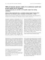
We now discuss the calculated isotherms on a p–v diagram. Figure 1
shows an isothermal line at 9300 K. To illustrate that the line is indeed
isothermal, the temperature at each point is also plotted. It is seen that
the temperature variation is within the range of 9300 ± 3 K. A liquid-
gas coexistence region can be identified in Fig. 1 where the pressure stays
constant. At the left side of the isotherm, the pressure decreases rapidly
with an increase of specific volume until it reaches 0.2898 ×10
−3
m
3
·kg

−1
(corresponding to a density of 3450 kg·m
−3
) and a pressure of 0.99 GPa,
Fig. 1. Isotherm at 9300 K.
14 Cheng and Xu
i.e., the point p =0.99 GPa, v =0.2898 ×10
−3
m
3
·kg
−1
, and T =9300 K is
a point on the liquid-gas saturation line. As the specific volume increases
further, the pressure remains constant. (A close examination of this pla-
teau reveals a very small van der Waals-like loop, which is due to the com-
putational size used. The van der Waals-like loop is more obvious when a
smaller calculation domain is used.) The pressure starts to decrease again
with an increase of the specific volume from v =0.5609 ×10
−3
m
3
·kg
−1
(corresponding to a density of 1783 kg·m
−3
). This indicates that the point
p =0.99 GPa, v =0.5609 ×10
−3
m

3
·kg
−1
is the other point on the liquid-
gas saturation line at T =9300 K. Between these two points, the material
is a mixture of liquid and gas states, although the mass fraction of each
phase changes with the specific volume.
The phases of the material along the isotherm are confirmed by the
observation of the atomic structures. In Fig. 2, the material structures cor-
responding to three states in Fig. 1 are shown. Each black dot in Fig. 2
represents one atom. The more uniform liquid and gas structures can be
seen from the atomic distribution in Figs. 2a (liquid) and c (gas), while
at state b, which is a mixture of liquid and gas, the material structure is
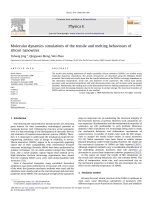
not as uniform. The difference in uniformity at these three states is also
shown in Fig. 3, the snapshot of atomic number density at different loca-
tions along the long axis of the calculation domain (39.66 nm at room
temperature). It is seen that the fluctuation of density at state b is larger
than those at the other two states, indicating the coexistence of gas and
liquid state in state b while the other two states have more uniform den-
sity throughout the calculation domain. However, it is seen from Fig. 2c
that the atomic distribution is not completely uniform, indicating that a
more complex structure may exist in the gaseous phase such as dimers and
higher-order clusters, particularly near the binodal line. This indicates that
Fig. 2. Atomic structure of (a) liquid, (b) liquid-gas coexistence, and (c) gas phases as
marked on the phase diagram in Fig. 1.
Molecular Dynamics Calculation of Critical Point of Nickel 15
0
a (liquid)
b (liquid + gas)
c (gas)

0
10
20
30
40
50
60
Atomic number density
x, nm
20 8040
60
Fig. 3. Atomic number density at several locations on
the phase diagram in Fig. 1 (a, liquid; b, liquid-gas coex-
istence; c, gas).
atomic distribution plots may not be a reliable way to determine the phase
of a material. Another way to distinguish the phases is to compute the
radial distribution functions at the locations of interest. The radial distri-
bution function describes the distribution of the distances between any two
atoms in the material, and it represents the relative probability to find a
pair of atoms separated by distance r. The definition of the radial distri-
bution function g(r) is given as
g
(
r
)
=

n
(
r +r

)
−n
(
r
)
4πr
2
r
V
N

(8)
where n(r) is the number of atoms within a distance r from a certain
atom, r is the distance step (chosen as 0.01 nm in this calculation to
achieve an appropriate resolution of g(r)), V is the total volume, and N
is the total atom number. The radial distribution function is always calcu-
lated and averaged for a large number of atoms.
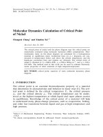
Typical radial distribution functions for solid, liquid, and gas of
nickel are shown in Fig. 4. Crystal solids have regular lattice structure, so
distances between atoms have a regular distribution which is represented
by oscillations of g(r) in both long and short ranges. For liquids, the
short-range order remains, but the long-range order disappears. Both the
short-range and long-range orders vanish for gases. Therefore, the radial
distribution, function is commonly used to illustrate the structure and the
phase of a material [8]. The radial distribution functions at states a, b,
and c in Fig. 1 are calculated and shown in Fig. 5. Note that the curves
of states b and c are raised for clarity. For state a, the radial distribution
16 Cheng and Xu
solid
liquid

gas
-0.5
0
0.5
1
1.5
2
2.5
3
3.5
0
g (r)
r, nm
short range
order
long range
order
0.2
0.4
0.6
0.8 1
1.2 1.4
Fig. 4. Radial distribution function for solid, liquid, and
gas.
0 0.2 0.4 0.6 0.8 1 1.2 1.4
a
b
c
g(r)
r, nm

short range order
Fig. 5. Radial distribution function g(r) at several loca-
tions on the phase diagram in Fig. 1 (a, liquid; b, liquid–
gas coexistence; c, gas). Curves of b and c are raised for
clarity.
function shows short-range order as that of a liquid. (The radial distribu-
tion function does not return to 1 at 1.4 nm, which is likely due to the
truncation error in the calculation.) For the radial distribution function at
state c, the short-range order disappears completely, which indicates that
state c is in the gas phase. The profile of g(r) for state b is between those
of a and c, and the short-range order is only observed partially.
Isotherms are also constructed for several other temperatures as
shown in Fig. 6. It is seen that at temperatures lower than 9450 K,
Molecular Dynamics Calculation of Critical Point of Nickel 17
Fig. 6. Calculated isotherms on p–v diagram around the
critical point.
Fig. 7. Isotherms calculated from MD simulations and
from the Redlich–Kwong equation.
there is always a liquid–gas coexistence region where the pressure does
not change with the specific volume. The boundaries of the liquid–gas
co-existence regions form the binode lines. When the temperature is higher
than 9500 K, the pressure decreases monotonically with an increase of the
specific volume and the plateau of pressure with respect to specific volume
does not exist. Therefore, the critical temperature lies between 9450 and
9500 K.
Further calculations at temperatures between 9450 and 9500 K found
that the parameters of the critical point are: T
c
=9460 ± 20 K, ρ
c

=2560±
100 kg·m
−3
, and p
c
=1.08 ± 0.01 GPa. There are only a few values in the
18 Cheng and Xu
literature for the critical point of nickel: 9576 K / 2293 kg·m
−3
/ 1.12 GPa
[11], 7810 K / 2210 kg·m
−3
/ 0.49 GPa [12], and 9100 ± 150 K / 0.9 ±0.1
GPa [13]. These values are either extrapolated from low-temperature data
using semi-empirical equations of state, or from shock-compression exper-
iments.
Another outcome of the MD results is the equation of state (EOS),
which is often unavailable at high temperature and high pressure. In this
calculation, we tried to obtain simple two-constant forms of an equation
of state, such as van der Waals, Redlich–Kwong, and Berthelot equations
and found that the Redlich–Kwong equation best matches the MD data.
The Redlich–Kwong equation has the form,
p =
nRT
v −b
−
a
v
(
v +b

)
√
T
(9)
where a and b are constants. These constants can be obtained from the
requirements that both the first and second derivatives of the isotherm are
zero at the critical point, which results in
a =0.42748
(
nR
)
2
T
5/2
c
p
c
,
b =0.08664
nRT
c
p
c
(10)
Using the critical point parameters obtained from MD, a and b are found
to be
a =69113 m
6
·kg
−2

·K
1/2
,b=1.0749 ×10
−4
m
3
·kg
−1
(11)
Using these values, Eq. (9) is plotted together with isotherms obtained
from MD calculations. For the isotherms calculated from Eq. (9), the sec-
tions between the binodes should be ignored. As mentioned earlier, the
Redlich–Kwong equation matches the MD results the best, while other
forms of the equation of state do not match MD results as well (not
shown in the figure).
4. CONCLUSION
In this work, the phase diagram of nickel near the critical point is cal-
culated using molecular dynamics simulations. Isotherms near the critical
temperature are constructed on a p–v diagram. Regions where liquid and
gas co-exist and the binode lines are obtained. The critical point obtained
in this work is in good agreement with literature values. It is also found
that the Redlich–Kwong equation can best represent the phase diagram
near the critical point compared with other forms of EOS.
Molecular Dynamics Calculation of Critical Point of Nickel 19
ACKNOWLEDGMENT
Support to this work by the National Science Foundation is gratefully
acknowledged.
REFERENCES
1. M. J. Moran and H. N. Shapiro, Fundamentals of Engineering Thermodynamics (John
Wiley & Sons, New York, 1996), pp. 72–74, 491.

2. Y. Guissani and B. Guillot, J. Chem. Phys. 104:7633 (1996).
3. D. O. Dunikov, S. P. Malyshenko, and V. V. Zhakhovskii, J. Chem. Phys. 115: 6623 (2001).
4. A. Shibinsky, S. V. Buldyrev, G. Franzese, G. Malescio, and H. E. Stanley, Phys. Rev. E
69:061206 (2004).
5. L. A. Girifalco and V. G. Weizer, Phys. Rev. 114:687 (1959).
6. S. M. Foiles, M. I. Baskes, and M. S. Daw, Phys. Rev. B 33:7983 (1986).
7. M. S. Daw, S. M. Foiles, and M. I. Baskes, Mater. Sci. Rep. 9:251 (1993).
8. M. P. Allen and D. J. Tildesley, Computer Simulation of Liquids (Clarendon Press, Oxford,
1987), pp. 78–80.
9. J. M. Haile, Molecular Dynamics Simulation: Elementary Methods (John Wiley & Sons,
New York, 1992), p. A1.
10. H. J. C. Berendsen, J. P. M. Postma, W. F. van Gunsteren, A. DiNola, and J. R. Haak,
J. Chem. Phys. 81:3684 (1984).
11. D. A. Young and B. J. Alder, Phys. Rev. A 3:364 (1971).
12. M. M. Martynyuk, Russ. J. Phys. Chem. 57:810 (1983).
13. D. N. Nikolaev, V. Y. Ternovoi, A. A. Pyalling, and A. S. Filimonov, Int. J. Thermophys.
23:1311 (2002).