- Trang chủ >>
- Cao đẳng - Đại học >>
- Luật
7 QC TOOLS OLD ( 7 Công Cụ Quản Lý Chất Lượng Cũ )
Bạn đang xem bản rút gọn của tài liệu. Xem và tải ngay bản đầy đủ của tài liệu tại đây (81.62 KB, 13 trang )
THE 7 QC TOOLS
1 Introduction
The 7 QC Tools are simple statistical tools used for problem solving.
These tools were either developed in Japan or introduced to Japan by the
Quality Gurus such as Deming and Juran. In terms of importance, these
are the most useful. Kaoru Ishikawa has stated that these 7 tools can be
used to solve 95 percent of all problems. These tools have been the
foundation of Japan's astomishing industrial resurgence after the second
world war.
The following are the 7 QC Tools :
1. Pareto Diagram
2. Cause & Effect Diagram
3. Histogram
4. Control Charts
5. Scatter Diagrams
6. Graphs
7. Check Sheets
2 Pareto Diagram
Pareto Diagram is a tool that arranges items in the order of the magnitude
of their contribution, thereby identifying a few items exerting maximum
influence. This tool is used in SPC and quality improvement for prioritising
projects for improvement, prioritising setting up of corrective action teams
to solve problems, identifying products on which most complaints are
received, identifying the nature of complaints occurring most often,
identifying most frequent causes for rejections or for other similar
purposes.
The origin of the tool lies in the observation by an Italian economist
Vilfredo Pareto that a large portion of wealth was in the hands of a few
people. He observed that such distribution pattern was common in most
fields. Pareto principle also known as the 80/20 rule is used in the field of
materials management for ABC analysis. 20% of the items purchased by
a company account for 80% of the value. These constitute the A items on
which maximum attention is paid.
Dr.Juran suggested the use of this principle to quality control for
separating the "vital few" problems from the "trivial many" now called the
"useful many".
Procedure :
The steps in the preparation of a Pareto Diagram are :
1. From the available data calculate the contribution of each individual
item.
2. Arrange the items in descending order of their individual contributions.
If there are too many items contributing a small percentage of the
contribution, group them together as "others". It is obvious that
"others" will contribute more than a few single individual items. Still it
is kept last in the new order of items.
3. Tabulate the items, their contributions in absolute number as well as in
percent of total and cumulative contribution of the items.
4. Draw X and Y axes. Various items are represented on the X-axis.
Unlike other graphs Pareto Diagrams have two Y-axes - one on the left
representing numbers and the one on right representing the percent
contributions. The scale for X-axis is selected in such a manner that
all the items including others are accommodated between the two Y-
axes. The scales for the Y-axes are so selected that the total
number of items on the left side and 100% on the right side occupy the
same height.
5. Draw bars representing the contributions of each item.
6. Plot points for cumulative contributions at the end of each item. A
simple way to do this is to draw the bars for the second and each
subsequent item at their normal place on the X-axis as well as at a
level where the previous bar ends. This bar at the higher level is
drawn in dotted lines. Drawing the second bar is not normally
recommended in the texts.
7. Connect the points. If additional bars as suggested in step 6 are
drawn this becomes simple. All one needs to do is - connect the
diagonals of the bars to the origin.
8. The chart is now ready for interpretation. The slope of the chart
suddenly changes at some point. This point separates the 'vital few'
from the 'useful many' like the A,B and C class items in materials
management.
An example of a Pareto Chart is given in Annexure - 1
3 Cause & Effect Diagram
A Cause-and Effect Diagram is a tool that shows systematic relationship
between a result or a symptom or an effect and its possible causes. It is
an effective tool to systematically generate ideas about causes for
problems and to present these in a structured form. This tool was devised
by Dr. Kouro Ishikawa and as mentioned earlier is also known as Ishikawa
Diagram.
Structure
Another name for the tool, as we have seen earlier, is Fish-Bone Diagram
due to the shape of the completed structure. If we continue the analogy,
we can term various parts of the diagram as spine or the backbone, large
bones, middle bones and small bones as seen in the structure of cause-
and-effect diagram.
The symptom or result or effect for which one wants to find causes is put
in the dark box on the right. The lighter boxes at the end of the large
bones are main groups in which the ideas are classified. Usually four to
six such groups are identified. In a typical manufacturing problem, the
groups may consist of five Ms - Men, Machines, Materials, Method and
Measurement. The six M Money may be added if it is relevant. In some
cases Environment is one of the main groups. Important subgroups in
each of these main groups are represented on the middle bones and
these branch off further into subsidiary causes represented as small
bones. The arrows indicate the direction of the path from the cause to the
effect.
Cause-and Effect diagram is a tool that provides best results if used by a
group or team. Each individual may have a few ideas for the causes and
his thinking is restricted to those theories. More heads are needed to
make a comprehensive list of the causes. Brainstorming technique is
therefore very useful in identifying maximum number of causes.
Procedure
The steps in the procedure to prepare a cause-and-effect diagram are :
1. Agree on the definition of the 'Effect' for which causes are to be found.
Place the effect in the dark box at the right. Draw the spine or the
backbone as a dark line leading to the box for the effect.
2. Determine the main groups or categories of causes. Place them in
boxes and connect them through large bones to the backbone.
3. Brainstorm to find possible causes and subsidiary causes under each
of the main groups. Make sure that the route from the cause to the
effect is correctly depicted. The path must start from a root cause and
end in the effect.
4. After completing all the main groups, brainstorm for more causes that
may have escaped earlier.
5. Once the diagram is complete, discuss relative importance of the
causes. Short list the important root causes.
An example of a cause and effect diagram is given in Annexure - 2
4 Histogram
Histograms or Frequency Distribution Diagrams are bar charts showing
the distribution pattern of observations grouped in convenient class
intervals and arranged in order of magnitude. Histograms are useful in
studying patterns of distribution and in drawing conclusions about the
process based on the pattern.
The Procedure to prepare a Histogram consists of the following steps :
1. Collect data (preferably 50 or more observations of an item).
2. Arrange all values in an ascending order.
3. Divide the entire range of values into a convenient number of groups
each representing an equal class interval. It is customary to have
number of groups equal to or less than the square root of the number
of observations. However one should not be too rigid about this. The
reason for this cautionary note will be obvious when we see some
examples.
4. Note the number of observations or frequency in each group.
5. Draw X-axis and Y-axis and decide appropriate scales for the groups
on X-axis and the number of observations or the frequency on Y-axis.
6. Draw bars representing the frequency for each of the groups.
7. Provide a suitable title to the Histogram.
8. Study the pattern of distribution and draw conclusion.
Stoppages due to Machines Problem
21
18
15
3
6
9
12
0. 1.
2.
3.
4. 5.
6. 7. 8. 9.
F
r
e
q
u
e
n
c
y
No. of Stoppages per shift
Diagram - 1
The Histogram is normal if the highest frequency is in the central group and there
is symmetrical tapering on either side of the central group as in diagram 1. The
natural or normal distribution would indicate that the process being studied is
under control. Let us see a few instances of Histograms that are not normal and
what conclusions one can drawn from them.
Diagram 2 shows two peaks with a little valley between them. Such a
distribution is known as Bimodal Distribution. It indicates that the lot being
examined is mixed. It may be due to pooling of production from two machines or
two shifts, each having a different central value. When one encounters such a
distribution, one should study the two lots separately if the identity of the two lots
can be ascertained. For instance if one is examining the dimensions of
containers and encounters bimodal distribution, the containers from the two
moulds can be separated by the mould mark on them. Segregating the data
from
High Plateau Bimodal Distribution
Diagram - 3 Diagram - 2
different lots is known as Stratification of data. We will see more about this soon.
Each lot may then exhibit a normal distribution. In that case one only needs to
find why the two lots are different and eliminate the cause. Diagram 3 shows a
High Plateau that reminds one of Empire State building. One often encounters
this type of distribution in incoming materials if the supplier has sorted out and
removed items showing wide variation. It can also occur in finished products if
there is inspection and sorting at the end of the production line. Such a
distribution indicates that the actual variation in the process is more than what is
seen in the Histogram. The items with wider variation have been removed before
sampling. Such a process generates waste, is uneconomical and needs to be
improved to reduce the variation.
Cliff pattern seen in Diagram 5 may arise due to inspection and sorting out the
items only at one end - those below a specific value, but not at the other end. It
can also occur when the lower end is zero, and the variation on the higher end
goes well beyond twice the value at the peak. Alternate peaks and vales as
shown in Diagram 4 is an unnatural pattern that may arise even if the process is
under control if the figures have been rounded off incorrectly or class intervals
have been selected wrongly. Examine the process of rounding of figures in the
data and regroup the data in correct classes and you may get a normal pattern.
A Histogram with an unnatural pattern may indicate that there is possibly
something unusual with the process, but is not an evidence of a process being
out of control. For instance a Histogram depicting the distribution of age of all
citizens will not peak at the centre. It will start with a cliff tapering gradually till
around the life expectancy then dropping a little faster and once again tapering
into along tail. The distribution of ages of students in a school shows a high
plateau as there is a specific age at which children are admitted into a school and
they would pass out of the school by a specific age. Still one needs to consider
the reasons for every unnatural pattern and draw conclusions based on the
pattern, one's knowledge about the process being studied and judgment based
on common sense.
Alternate Peaks and Vales
Diagram - 5
Diagram - 4
Cliff Pattern
5 Control Charts
Variability is inherent in all manufacturing processes. These variations
may be due to two causes ;
i. Random / Chance causes (un-preventable).
ii. Assignable causes (preventable).
Control charts was developed by Dr. Walter A. Shewhart during 1920's while he
was with Bell Telephone Laboratories.
These charts separate out assignable causes.
Control chart makes possible the diagnosis and correction of many production
troubles and brings substantial improvements in the quality of the products and
reduction of spoilage and rework.
It tells us when to leave a process alone as well as when to take action to correct
trouble.
BASIC CONCEPTS :
a. Data is of two types :
Variable - measured and expressed quantitatively
Attribute - quanlitative
b. Mean and Range :
⎯X - Mean is the average of a sub-group
R - Range is the difference between the minimum and maximum in a
sub-group
c. Control Charts for Variables
Charts depleting the variations in ⎯X and R with time are known as ⎯X and R
charts. ⎯X and R charts are used for variable data when the sample size of the
subgroup is 2-5. When the subgroup size is larger, s Charts are used instead of
R charts where s is the standard deviation of the subgroup.
d. Control Charts for Attributes
The control charts for attributes are p-chart, np-chart, c-chart and u-chart. Control
charts for defectives are p and np charts. P charts are used when the sample
size is constant and np charts are used when the sample size is variable. In the
case where the number of defects is the data available for plotting, c and u charts
are used. If the sample size is constant, c charts are used and u charts are used
for variable sample sizes.
6 Scatter Diagram
When solving a problem or analysing a situation one needs to know the
relationship between two variables. A relationship may or may not exist between
two variables. If a relationship exists, it may be positive or negative, it may be
strong or weak and may be simple or complex. A tool to study the relationship
between two variables is known as Scatter Diagram. It consists of plotting a
series of points representing several observations on a graph in which one
variable is on X-axis and the other variable in on Y-axis. If more than one set of
values are identical, requiring more points at the same spot, a small circle is
drawn around the original dot to indicate second point with the same values. The
way the points lie scattered in the quadrant gives a good indication of the
relationship between the two variables. Let us see some common patterns seen
in Scatter Diagrams and the conclusions one can draw based on these patterns.
Diagrams 6 to 11 show some of the more common patterns.
Diagram 6 shows a random distribution of points all over the quadrant. Such a
distribution or scatter indicates a lack of relationship between the two variables
being studied. In Diagram 7, the points appear scattered closely along a line
(shown as a dotted line in the diagram) travelling from the Southwest to the
Northeast direction indicating that if the variable on X-axis increases, the variable
on Y-axis also increases. This is a positive relationship. As the points are very
closely scattered around the straight line, the relationship is said to be strong.
Diagram 8, in which the points are scattered closely around a line sloping in
Northwest to Southeast direction, indicates a strong negative relationship. A
negative relationship means that the variable on Y-axis goes down as the
variable on X-axis goes up. Diagrams 9 and 10 shows a scatter of points loosely
spread around lines in directions similar to Diagrams 10 and 8 respectively.
Hence scatter in Diagram 9 indicates a weak positive relationship and that in
Diagram 10 indicates a weak negative relationship. Weak relationship means
that the variables are related but there are possibly other factors besides the
variable on X-axis also affecting the variable on Y-axis. If other factors are kept
constant in a controlled experiment and the data is again plotted, it would result
in a scatter showing a strong relationship. Diagrams 7 to 10 showed a simple
linear relationship between the two variables over the entire range. Very often
the relationship is not that simple. The variable on Y-axis may increase up to a
point as the variable on X-axis is increased but after that it may stay the same or
even decrease. Diagram 11 shows one such complex scatter.
y
y
y
y
y
y
y
y
y
y
y
y
y
y
y
y
y
y
y
y
y
y
y
y
y
y
y
y
y
y
y
y
y
y
y
y
y
y
y
y
y
y y
y
y
y
y
y
y
y
y
y
~
y
y
y
y
~
y
y
y
y
y
~
~
y
y
~
y
~
y
y
y
y
y
y
Diagram - 7
Diagram - 6
y
y
y
y
y
y
y
y
y
y
y
y
y
y
y
y
y
y
y
y
y
y
y
y
y
y
y
y
y
y
y
Diagram - 9
y
y
y
y
y
y
y
y
y
y
y
y y
y
y
y
y
~
~
~
y
y
y
y
y
y
y
y
y
y
y
Diagram - 8
y
y
y
y
y
y
y
y
y
y
y
y
y y
y
y
y
y
y
y
y
y
y
y
y
y
y
y
y
y
Diagram - 10
Diagram - 11
y
y
y
y
y
y
y
y
y
y
y
y
y
y
y
y
y
y
y
y
y
y
y
y
y
y
y
y
y
y
y
y
y
y
y
yy
y
2.7 Graphs
Graphs of various types are used for pictoral representation of data.
Pictoral representation enables the user or viewer to quickly grasp the
meaning of the data. Different graphical representation of data are
chosen depending on the purpose of the analysis and preference of the
audience. The different types of graphs used are as given below :
S.No Type of Graph Purpose
1. Bar Graph To compare sizes of data
2. Line Graph To represent changes of data
3. Gantt Chart To plan and schedule
4. Radar Chart To represent changes in data (before
and after)
5. Band Graph Same as above
6. Pie Chart Used to indicate comparative weights
7. ISO Graph To represent data using symbols
8 Check Sheets
8.1 As measurement and collection of data forms the basis for any analysis,
this activity needs to be planned in such a way that the information
collected is both relevant and comprehensive.
8.2 Check sheets are tools for collecting data. They are designed specific to
the type of data to be collected. Check sheets aid in systematic collection
of data. Some examples of check sheets are daily maintenance check
sheets, attendance records, production log books, etc.
9. Stratification
Data collected using check sheets needs to be meaningfully classified.
Such classification helps gaining a preliminary understanding of relevance
and dispersion of the data so that further analysis can be planned to
obtain a meaningful output. Meaningful classification of data is called
stratification. Stratification may be by group, location, type, origin,
symptom, etc.
Some Examples :
a) Data on rejected product may be classified either machine wise or
operator wise or shift wise.
b) Data of production of food grains may be classified nation wise, state
wise or district wise, etc.
c) Voting percentages may be classified party wise, state wise,
community wise or gender wise, etc.
Compiled from D L Shah Trust publication
By B.Girish, Dy. Director
National Productivity Council, Chennai
PARETO DIAGRAM
0
3
1.1
0.8
0.7
0.4
7.8
14
12
2
4
6
8
10
100%
No. of defects
Percentage (%)
50
Pareto Diagram showing the break-down of Defects
Annexure - 1
MAN
MATERIALS
Under trained
Loose
( 1)
Open Digits
METHOD
MACHINE
Poor
Workmanship
Improper Fixing of
Wires at Connector
Wrong Orientation
of Wires at
Connector
Poor Workmanship at
Camping
P
e
r
so
n
Wrong Orientation of
Wires at soldering
Wrong Orientation
of PCB
Poor Solderin
Pin
Broken
Wir
es
g
Improper Taping
of Units
Cold
ering
Tester Malfunctioning
Contact Problem
Solder Bridging
Unsoldered Leads
Wave Solder
Improper Striping of
Wires
amping of
Connectors
Camping Machine
Malfunctioning
Trace
Broken
Connector
Defective PCB
Defective
Displays
Position of
Ta
Broken
Improper C
Sold
Excessive
Ta
p
in
g
p
es
Annexure - 2