Astm stp 1421 2002
Bạn đang xem bản rút gọn của tài liệu. Xem và tải ngay bản đầy đủ của tài liệu tại đây (6.97 MB, 390 trang )
STP 1421
Outdoor Atmospheric Corrosion
Herbert E. Townsend, editor
ASTM Stock Number: STPI421
ASTM
100 Barr Harbor Drive
West Conshohocken, PA 19428-2959
INTERNATIONAL
Printed in the U.S.A.
Library of Congress Cataloging-in-Publication Data
Outdoor atmospheric corrosion / Herbert E. Townsend, editor.
p. cm.--(STP ; 1421)
"ASTM Stock Number: STP1421."
Includes bibliographical references and index.
ISBN 0-8031-2896-7
1. Corrosion and anti-corrosives--Congresses. I. Townsend, Herbert E., 1938ASTM special technical publication ; 1421
I1.
TA418.74 .O88 2002
620.1'1223--dc21
2002074627
Copyright 9 2002 AMERICAN SOCIETY FOR TESTING AND MATERIALS INTERNATIONAL, West
Conshohocken, PA. All rights reserved. This material may not be reproduced or copied, in whole or
in part, in any printed, mechanical, electronic, film, or other distribution and storage media, without
the written consent of the publisher.
Photocopy Rights
Authorization to photocopy items for internal, personal, or educational classroom use, or
the internal, personal, or educational classroom use of specific clients, is granted by the
American Society for Testing and Materials International (ASTM) International provided that
the appropriate fee is paid to the Copyright Clearance Center, 222 Rosewood Drive, Danvers,
M A 01923; Teh 978-750-8400; online: />
Peer Review Policy
Each paper published in this volume was evaluated by two peer reviewers and at least one editor. The authors addressed all of the reviewers' comments to the satisfaction of both the technical
editor(s) and the ASTM International Committee on Publications.
To make technical information available as quickly as possible, the peer-reviewed papers in this
publication were prepared "camera-ready" as submitted by the authors.
The quality of the papers in this publication reflects not only the obvious efforts of the authors
and the technical editor(s), but also the work of the peer reviewers. In keeping with long-standing
publication practices, ASTM International maintains the anonymity of the peer reviewers. The ASTM
International Committee on Publications acknowledges with appreciation their dedication and contribution of time and effort on behalf of ASTM International.
Printed in Phila., PA
August 2002
Foreword
This publication, Outdoor Atmospheric Corrosion, contains papers presented at the symposium of the same name held in Phoenix, Arizona, on 8-9 May 2001. The symposium was
sponsored by ASTM International Committee G1 on Corrosion of Metals. The symposium
co-chairman was Herbert E. Townsend, Consultant, Center Valley, PA.
Dedication to Seymour K. Coburn
1917-2001
This volume is dedicated to the memory of Seymour K. Coburn, who passed away on
January 4, 2001.
Sy, as he was known to many of his friends, was born in Chicago in 1917. He received
a BS in Chemistry from the University of Chicago in 1940, and an MS from Illinois Institute
of Technology in 1951. After initially working for Minor laboratories, Lever Brothers, and
the Association of American Railroads, he began a long career as a corrosion specialist at
the Applied Research Laboratories of US Steel Corporation.
Working with C. P. Larabee at US Steel, he became well known throughout the industry
for pioneering their studies of the effects of alloying elements on the corrosion of steels. To
do this, they studied the corrosion performance of hundreds of steel compositions exposed
to rural, marine, and industrial environments, and defined the beneficial effects of copper,
nickel, phosphorus, chromium, and silicon. No treatment of the subject is complete without
a reference to their classic paper, "The Atmospheric Corrosion of Steels as Influenced by
Changes in Chemical Composition," that was presented in 1961 to the First International
Congress on Metallic Corrosion in London.
Sy went on to become one of the leading advocates of weathering steels, that is, lowalloy steels which develop a protective patina during exposure in the atmosphere so that they
become corrosion-resistant without painting for use in applications such as bridges, utility
towers, and buildings. He was US Steel's research consultant for the John Deere Headquarters
on Moline, IL, the first building constructed with weathering steel, as well as the Chicago
Civic Center, and some of the first unpainted weathering steel bridges.
In 1970, he was transferred to the Special Technical Services unit of US Steel's Metallurgical Department where he became the top promoter and trouble-shooter for bridges and
other weathering steel applications. But it was not until he attended a workshop of the Steel
Structures Paint Council that he achieved his real goal in life--he became a teacher.
An active member of ASTM International, Sy chaired Subcommittee GI.04 on Atmospheric Corrosion from 1964 to 1970, and was instrumental in organizing this subcommittee.
He also was the prime mover in organizing and editing STP 646, "Atmospheric Factors
Affecting the Corrosion of Engineering Materials," and he chaired the symposium that led
to that STP, a celebration of 50 years of exposure testing at the State College, PA, ASTM
International atmospheric corrosion test site in May 1976.
After retiring in 1984, he continued to teach and actively consult around the world in
matters related to weathering steels and protective coatings. In addition to his ASTM International activities, Sy was also a member of the American Chemical Society, The American
Society for Metals, the National Association of Corrosion Engineers, and the Steel Structures
Painting Council.
Stan Lore
612 Scrubgrass Road
Pittsburgh, PA 15243
Contents
Overview
xi
PREDICTION OF O U T D O O R CORROSION PERFORMANCE
Analysis of Long-Term Atmospheric Corrosion Results from ISO CORRAG
Programms. w. DEAN AND D. B. REISER
Corrosivity Patterns Near Sources of Salt Aerosols~R. o. KLASSEN,
P. R. ROBERGE, D. R. LENARD, AND G. N. BLENKINSOP
19
Field Exposure Results on Trends in Atmospheric Corrosion and Pollution-J. TIDBLAD, V. KUCERA, A. A. MIKHAILOV, M. HENRIKSEN, K. KREISLOVA,
T. YATES, AND B. SINGER
34
Time of Wetness (TOW) and Surface Temperature Characteristics of
Corroded Metals in Humid Tropical Climate--L. VELEVAAND
A. A L P U C H E - A V I L E S
Analysis of ISO Standard 9223 (Classification of Corrosivity of Atmospheres)
in the Light of Information Obtained in the Ibero-American Micat
Project~M. M O R C I L L O , E. A L M E I D A , B. CHICO, AND D. DE LA FUENTE
48
59
Improvement of the ISO Classification System Based on Dose-response
Functions Describing the Corrosivity of Outdoor Atmospheres~
J. TIDBLAD, V. KUCERA, A. A. MIKHAILOV, AND D. K N O T K O V A
73
NO 2 Measurements in Atmospheric Corrosion Studies---c. ARROYAVE,
F. ECHEVERRIA, F. HERRERA, J. D E L G A D O , D. A R A G O N , AND M. M O R C I L L O
88
The Effect of Environmental Factors on Carbon Steel Atmospheric Corrosion;
The Prediction of Corrosion--L. T. H. LIENAND P. T. SAN
103
Classification of the Corrosivity of the Atmosphere~Standardized
Classification System and Approach for AdjustmentmD. KNOTKOVA,
V. KUCERA, S. W. DEAN, AND P. BOSCHEK
109
LABORATORY TESTING AND SPECIALIZED O U T D O O R TEST M E T H O D S
ln-situ Studies of the Initial Atmospheric Corrosion of IronmJ. WEISSENRIEDER
A N D C. L E Y G R A F
127
Effect of Ca and S on the Simulated Seaside Corrosion Resistance of
1.0Ni-0.4Cu-Ca-S Steel--J. Y. roD, w. v. CHOO, AND i . YAMASHITA
139
Effect of C # + and So42- on the Structure of Rust Layer Formed on Steels by
Atmospheric Corrosion--M. Y A M A S H I T A , H. UCHIDA, AND O. C. C O O K
149
Analysis of the Sources of Variation in the Measurement of Paint C r e e p - E. T. McDEVITT AND F. J. FRIEDERSDORF
Atmospheric Corrosion Monitoring Sensor in Outdoor Environment Using AC
Impedance Technique---H. K A T A Y A M A , M. Y A M A M O T O , AND T. K O D A M A
157
171
EFFECTS OF CORROSION PRODUCTS ON THE ENVIRONMENT
Environmental Effects of Metals Induced by Atmospheric Corrosion-185
1. O. WALLINDER A N D C. L E Y G R A F
Environmental Effects of Zinc Runoff from Roofing Materiais--A New
Muitidisciplinary Approach--s. BERTLING, I. O. W A L L I N D E R , C. L E Y G R A F
200
AND D. BERGGREN
Runoff Rates of Ziuc--A Four-Year Field and Laboratory Study--w. HE,
216
I. O. WALLINDER, AND C. L E Y G R A F
Atmospheric Corrosion of Naturally and Pre-Patinated Copper Roofs in
Singapore and Stockholm--Runoff Rates and Corrosion Product
Formation--i. o. WALLINDER, T. KORPINEN, R. S U N D B E R G , AND C. L E Y G R A F
230
Environmental Factors Affecting the Atmospheric Corrosion of C o p p e r - S. D. C R A M E R , S. A. MATTHES, B. S. COVINO, JR., S. J. B U L L A R D , AND
245
G. R. HOLCOMB
Precipitation
Runoff
From
Lead--s.
A. MATTHES, S. D. C R A M E R , B. S. COVINO,
JR., S. J. BULLARD, AND G. R. H O L C O M B
265
LONG-TERM OUTDOOR CORROSION PERFORMANCE
OF E N G I N E E R I N G M A T E R I A L S
Evaluation of Nickel-Alloy Panels from the 20-Year ASTM G01.04
Atmospheric Test Program Completed in 1996--E. L. HmNER
277
Twenty-One Year Results for Metallic-Coated Steel Sheet in the ASTM 1 9 7 6
Atmospheric Corrosion Tests--H. E. TOWNSENDAND H. H. LAWSON
284
Estimating the Atmospheric Corrosion Resistance of Weathering Steels-H. E. TOWNSEND
292
P e r f o r m a n c e of W e a t h e r i n g Steel T u b u l a r S t r u c t u r e s - - M . L. HOITOMT
301
A t m o s p h e r i c Corrosion a n d W e a t h e r i n g Behavior of Terne-Coated Stainless
Steel R o o f i n g - - m M. KAIN A N D P. W O L L E N B E R G
316
O u t d o o r A t m o s p h e r i c Degradation of Anodic a n d P a i n t Coatings on
A l u m i n u m in Atmospheres of I b e r o - A m e r i c a m M . MORCJLLO,
J. A. G O N Z A L E Z , J. S I M A N C A S , A N D F. C O R V O
329
1940 ' T i l N o w m L o n g - T e r m M a r i n e A t m o s p h e r i c C o r r o s i o n Resistance of
Stainless Steel a n d O t h e r Nickel Containing A i l o y s - - m M. KAIN,
B. S. P H U L L , A N D S. J. PIKUL
343
Twelve Year A t m o s p h e r i c Exposure Study of Stainless Steels in C h i n a - C. LIANG AND W. HOU
358
Effects of Alloying on A t m o s p h e r i c Corrosion of S t e e l s - - w . HOU AND C. LIANG
368
A u t h o r Index
379
S u b j e c t Index
381
Overview
This book is a collection of papers presented at the ASTM International Symposium on
Outdoor and Indoor Atmospheric Corrosion that was held in Phoenix, AZ in May 2001.
With presentations from authors representing ten counties in North and South America,
Europe, and Asia, the symposium was truly international.
The symposium was originally conceived as a vehicle to present results of the 1976 ASTM
International outdoor atmospheric corrosion test program. During the initial scheduling, it
was combined with another symposium being planned by Robert Baboian on indoor corrosion to form a joint symposium on both outdoor and indoor corrosion. Although a joint
symposium was organized accordingly, contributions on the indoor topic did not materialize.
Consequently, this STP is devoted entirely to the outdoor topic.
Corrosion of metals in the atmosphere has been an important topic for many years, as
evidenced by the many symposium volumes previously published by ASTM International.
9 STP 67, Symposium on Atmospheric Exposure Tests on Nonferrous Metals, 1946.
9 STP 175, Symposium on Atmospheric Corrosion of Non-Ferrous Metals, 1956.
9 STP 290, Twenty-Year Atmospheric Investigation of Zinc-Coated and Uncoated Wire
and Wire Products, 1959.
9 STP 435, Metal Corrosion in the Atmosphere, 1968.
9 STP 558, Corrosion in Natural Environments, 1974.
9 STP 646, Atmospheric Factors Affecting the Corrosion of Engineering Materials, 1978,
S. K. Coburn, Editor.
9 STP 767, Atmospheric Corrosion of Metals, 1982, S. W. Dean, Jr. and E. C. Rhea,
Editors.
9 STP 965, Degradation of Metals in the Atmosphere, 1988, S. W. Dean, Jr. and T. S.
Lee, Editors.
9 STP 1239, Atmospheric Corrosion, 1995, W. W. Kirk and Herbert H. Lawson, Editors.
9 STP 1399, Marine Corrosion in Tropical Environments, 2000, S. W. Dean, Jr., Guillermo Hernandez-Duque Delgadillo, and James B. Bushman, Editors.
The present volume can be viewed as the most recent in a series on a topic of continuing
economic and ecological significance. As previously discussed (see "Extending the Limits
of Growth through Development of Corrosion-Resistant Steel Products," Corrosion, Vol. 55,
No. 6, 1999, 547-553), controlling losses of the world's resources due to atmospheric corrosion may be an important component of continuing economic development. Four major
themes are evident in this collection.
Prediction of Outdoor Corrosion Performance
One theme focuses on prediction of atmospheric corrosion performance from climatic data,
particularly in relation to methods being developed by the International Standards Organization (ISO). These attempt to classify the corrosivity of a location based either on shortterm exposure of standard coupons, or on local time of wetness, and deposition rates of
chloride and sulfate. Many of the assumptions in developing the ISO methodology are now
being reconsidered in the light of recently completed testing, and work continues to improve
the models.
xii
OUTDOOR ATMOSPHERIC CORROSION
Laboratory and Specialized Outdoor Test Methods
A second theme considers laboratory tests related to outdoor corrosion, and specialized
outdoor methods. These include methods of evaluating the results of outdoor tests, ways to
predict outdoor performance based on laboratory tests, and on work to develop a seaside
(salt-resistant) steel by additions of calcium and sulfur.
Effects of Corrosion Products on the Environment
A third theme examines the ecological effects of corrosion product runoff, a subject that
blends corrosion science, environmental technology, analytical chemistry and politics. Contributions from the Swedish Royal Institute of Technology, and the US Department of Energy
reflect a growing concern in developed countries for the ecological effects of dissolved
metals.
Long-Term Outdoor Corrosion Performance of Engineering Materials
The fourth theme is the documentation of the actual long-term outdoor behavior of engineering materials. This topic includes reports of the 21-year results of the 1976 ASTM
International outdoor atmospheric corrosion test program on nickel alloys, Galvalume, galvanized, and aluminum-coated steel sheet. Articles on the performance of unpainted, lowalloy weathering steel include a survey of utility poles in a wide range of environments,
work to establish a lean-alloy (Cu-P) grade as an inexpensive alternative to A588A, and the
development of a new ASTM GI01 corrosion index for estimating relative corrosion resistance from composition.
I am indebted to many for support and to the success of the symposium and this book.
These include the members of the Atmospheric Corrosion Subcommittee G 1.04, symposium
co-chairman Robert Baboian, a plethora of skilled reviewers, the presenters and authors of
a large number of high-quality papers, and the help of ASTM International staff including
Dorothy Fitzpatrick, Annette Adams, and Maria Langiewicz. This book, like the symposium,
is dedicated to the memory of Seymour Coburn, a pioneer in the development of weathering
steels, and an active contributor to the efforts of ASTM International in the field of outdoor
atmospheric corrosion.
Herbert E. Townsend
Consultant
Center Valley, PA
symposium co-chair and editor
PREDICTION OF O U T D O O R
CORROSION P E R F O R M A N C E
Sheldon W. Dean 1 and David B. Reiser2
Analysis of Long-Term Atmospheric Corrosion Results from ISO CORRAG
Program
Reference: Dean, S. W. and Reiser, D. B., "Analysis of Long-Term Atmospheric
Corrosion Results from ISO CORRAG Program," Outdoor Atmospheric Corrosion,
ASTM STP 1421, H. Townsend Ed., American Society for Testing and Materials
International, West Conshohocken, PA, 2002.
Abstract: A series of regression analyses was made on the multi-year corrosion losses of
panels of steel, zinc, copper, and aluminum in the ISO CORRAG program. In every
case, the only sites selected for the analyses were sites with all four exposures reported
and complete data sets on the time of wetness, sulfur dioxide, and chloride deposition.
The regressions with significant R values were then selected for further analyses. The
time exponent and one-year corrosion coefficient were regressed against the
environmental variables. None of the exponent regressions showed large environmental
effects. The steel exponent was increased by chloride deposition and time of wetness.
The copper exponent was increased by increasing time of wetness and decreased by
increasing chloride. Neither zinc nor aluminum exponents showed significant effects
from the environmental data. The best environmental regressions were only able to
predict the measured corrosion losses to within a factor of two for steel, zinc, and copper.
The aluminum loss predictions were worse. Some other environmental variables will
need to be found to improve this approach to predicting atmospheric corrosion.
Keywords: atmospheric corrosion, time of wetness, chloride deposition, sulfation, sulfur
dioxide deposition, ISO CORRAG program, regression analysis, time exponent
Introduction
Atmospheric corrosion is a major problem in the application of engineering metals
in many types of service. This form of deterioration has been noted from antiquity, but
the development of modern smelting and refining operations of steel has made the
economic consequences of atmospheric corrosion very significant in modern times. As a
result, there has been an ongoing effort to understand this phenomenon and to develop
standards that can be used to predict the severity of the process in service [1].
These concerns caused the International Organization for Standardization (ISO), at
the organization meeting of Technical Committee 156 in Riga, Latvia in 1976, to identify
atmospheric corrosion as a priority area for standards development. At the next meeting
1President, Dean CorrosionTechnology, 1316Highland Court, Allentown,Pennsylvania, 18103.
2 Lead Materials Engineer, CorporateEngineering Department, Air Products and Chemicals,Inc. 7201
HamiltonBoulevard,Allentown,Pennsylvania, 18195-1501.
Copyright9 2002 by ASTM lntcrnational
3
www.astm.org
4
OUTDOORATMOSPHERIC CORROSION
of TCl56 in Borhs, Sweden in 1978, the committee decided to form a working group
(TC 156/WG4) to develop standards for the classification of corrosion under the
leadership of members from the Czech Republic. As a result of this effort, four standards
were promulgated: ISO 9223, 9224, 9225, and 9226. These standards were based on an
extensive review of atmospheric corrosion results in Europe and North America [2].
The ISO CORRAG Collaborative Exposure Program was instituted in 1986 for the
purpose of establishing a worldwide program through ISO/TC 156 that would use
consistent standards, uniform exposure times, and standard materials. In addition, data
was to be obtained on temperature, humidity, sulfur dioxide concentrations, and chloride
deposition at 51 sites. Mass loss data was to be obtained on four metals: carbon steel,
zinc, copper, and aluminum using flat panels, 100 x 150 ram, and wire helices, 2-3 mm
diameter and 1 m long. Specimen removals were planned with six removals after oneyear exposures, one two-year, one four-year, and one eight-year. Three replicate
specimens of each metal and specimen type were to be removed at the end of each
interval. The one-year specimen exposures were to be spaced at six-month intervals [3].
The program has now been closed, and the results are being analyzed. Several
studies have been published comparing the relative performance of metals at different
sites [4]. The comparability of the panels and helices [5] and the predictability of
corrosion rates based on atmospheric variables have been published [6]. However, these
studies have focused on the one-year results and little attention has been given to the
multi-year specimens. The purpose of this paper is to examine the multi-year exposure
data to understand better the kinetics of the process and to determine to what degree the
atmospheric variables of time of wetness, sulfation, and chloride deposition can be used
to predict multi-year corrosion.
Procedures and Results
Input Data
The ISO CORRAG program has been described in detail earlier. The program
consisted of six one-year exposures of flat panels (100x 150x2 ram) and helix specimens
beginning every six months for three years. Multi-year exposures of two, four, and eight
years were initiated at the beginning of the exposure period. Triplicate specimens were
used for each exposure. The metals selected were a low carbon steel from a single
supplier and commercially pure zinc, copper, and aluminum. These nonferrous metals
were obtained from local sources in each of the participating nations. There were 51 sites
in 14 nations at the end of the program. The program was initiated in 1986 and officially
closed in 1998. At the conclusion of each exposure, the specimens were retrieved and
sent to the laboratory that had done the initial weighing for cleaning and evaluation.
Mass loss values were obtained and converted to corrosion thickness loss values in/.tm
units. The results from the various sites have been collected and tabulated by the Czech
member, SVUOM, and reported previously [6].
DEAN AND REISER ON ISO CORRAG PROGRAM
5
Data Analysis
The mass loss values were averaged for each exposure. In the case o f the one-year
results, the averages o f the data from all six exposures were used in this study. Average
values were calculated for time o f wetness (TOW), hrs./year, sulfur dioxide concentration
(SO2), mg/m 3, and chloride deposition rate (C1), mg/m 2 day for the eight-year period.
Only the sites with complete data on these variables were included in this study.
Regression analyses were carried lout for the fiat panel specimens at each site. The
mass loss data was converted to logarithmic values (base 10) and regressed against the
logarithmic exposure time in years as the independent variable. Previous studies have
found that atmospheric corrosion kinetics follow a power law relationship
M = aT b
(1)
where M = mass loss per unit area,
T = exposure time,
a = mass loss in the first year, and
b = mass loss time exponent (referred to as "slope").
This expression becomes as follows after the logarithmic conversion
logM = a' + b logT
(2)
where a' = log a (referred to as "intercept").
The Microsoft Excel 2000 spreadsheet program was used to carry out the regressions.
The correlation coefficient, R, is a measure o f the goodness of fit o f a regression, and the
value o f R 2 represents the fraction o f total variance o f the data explained by the regression.
For this study, there were only four exposure ~eriods so that the degrees o f freedom o f the
regression are two. The minimum value of R for a 5% significance level (95% confidence
level) is 0.83. The regressions with values below this level were excluded from the
analysis. This left 22 sites for steel, 23 for zinc and copper, and 21 for aluminum. The
results o f these regressions are plotted in Figure 1.
The values of a' and b from these regressions were then averaged and the standard
deviations were calculated for each metal and are shown in Table 1. The values were
plotted on probability paper to determine whether the values were normally distributed.
Correlation analyses were performed to determine if there was any correlation between
the a' and b values. The results of these analyses indicated that the distribution was
normal, and there was no significant correlation between a' and b. The correlation
coefficients are reported in Table 1.
6
OUTDOORATMOSPHERIC CORROSION
. . . . . . . . . . . . . .
!
[ .
.
.
.
.
.
!
1
I
0.8
.
S t e e l ,
.
.
.
.
.
.
.
.
:
Zinc
1.8
!
d
i
i
J
c,
om 0.6
t
9i
0.4
9i
"
~
...... A'. . . . . . . .
m
~1.6
Q
c
.
Z
E
"i
9-~ 1.4
0.2
1.2
-0.2
ii :
i
-0.4
0.2
0.4
0.6
0.8
Regression Slope: b
. . . . . . . . . . . . . . . . . . . . . . . . . . . . . . . . . . . .
_
0.4
1
! L
i i
J
I
i
0.6
0.8
1
1.2
Regression Slope: b
0.8
0.4
0.2
0.6
(u
o)
o 0.4
r -0.2
.9o
~.Q -0.4
~
c
o
-0.6
0.2
r
.9
-o.8
o
o
-1.2
-0.2
t
-1.4
t
-0.4
0.2
0.4
0.6
i
i
0.8
Regression Slope: b
.iI k
,I
Figure
1
-1.6
0.2
0.4
0,6
0.8
Regression Slope: b
X. ......
Results of regression analyses on mass loss vs. exposure time using
logarithmic conversion of the data.
1
1.2
DEAN AND REISER ON ISO CORRAG PROGRAM
Table 1 - Regression summary for log mass loss vs. log exposure time
Metal
Fe
Zn
Cu
Slope Ave
0.523
0.813
0.667
SD
0.121
0.143
0.142
Log Int Ave
1.556
0.194
0.160
SD
0.198
0.272
0.264
N
22
23
23
R
.186
0.125
0.322
c~) Plot of points on probability paper shows abnormality at ends
R=Correlation coefficient between slope and Log Int values
(>0.423 at 95% confidence level, DF=20)
A1
0.728
0.181
-.439 (~)
0.376
21
-0.222
Regression analyses were then carried out to determine to what degree the
measured environmental variables affected the a' and b values. Previous studies have
shown that the environmental variables have a strong effect on the a' value, but there
have been no studies of environmental variables on the b value. The results of these
regressions are shown in Tables 2A-D. In each case, regressions were made using all
three variables and then two at a time and finally single variable regressions. The reason
for this procedure was to attempt to eliminate variables that are not significant
contributors to the relationship.
Finally, it was desired to determine how closely the best expression was to matching
the measured eight-year corrosion losses. For each of the four metals, the regression
analyses for slope and intercept that yielded the smallest standard error were chosen. The
environmental variables were used in these expressions to predict the eight-year metal loss.
These calculations were made in each case. The first was based on the regression
expression used to fit the data from the exposures. The second was based on
environmental measurements and used predicted values for slope and intercept based on
Tables 2A-D. The third calculation used the measured one-year value and a predicted
slope from the regression in Tables 2A-D and environmental data. These results are shown
in Figure 2.
Discussion
Equation 1 has been widely used to describe the atmospheric corrosion kinetics [7].
The "a" term represents the corrosion loss in one year, while the "b" term represents the
long-term performance with "b" values less than one in most cases. Previous studies [6]
have focused on the effects environmental variables have on the one-year results but have
not considered the longer-term performance. Townsend [8] has examined the performance
of weathering steel and has discovered that alloying dements can, in some cases, change
the "b" value significantly. The lower the "b" is, the more protective the corrosion product
layer on the metal surface. The results in Figure 1 demonstrate clearly that the "b" values
show a significant variation for all four alloys. It was of interest to try to understand how
environmental variables affect the "b" value in this case of a single composition exposure.
8
OUTDOOR ATMOSPHERIC CORROSION
Table 2A - Summary of regression analyses on ,dope and intercept values with
environmental variable steel - 22 data points,
Regression
Variables
SO2,TOW,
CI
SO2, TOW
TOW, C1
SO2, C1
SO2
TOW*
C1
Slope Regressions
TOW (2)
S02 O)
Coef
t
Coef
t
CI (3)
Coef
t
lnt (4)
R2
SE
F
0,236
0.114
1.85
2.16
0.23
6.22
2.33
-1.37
-0.80
0.319
0.209
0.234
0,005
0,000
0,207
0.004
0.113
0.111
0.126
0.124
0.110
0.123
2.51
2.90
0.04
0.01
5.21
0.09
2.20
....
0.85
0.74
. . .
.....
0.24
5.24
6.19
. . .
. .
5.20
. . .
2.24
2.38
.
. . .
2.28
.
. . .
-1.37
0.49
. . .
. . .
0.48
.
-0.82
0.29
0.341
0.327
0.516
0.520
0.348
0.519
0.08
0.07
.
Intercept Regressions
S02 (~)
TOW (2)
Coef
t
Coef
t
.
0.29
C! O)
R2
SE
int (4)
F
Regression
Coef
t
Variables
2.37 0.69 4.92 2.22
6.66
41.9
3.50
1.316
SO2,TOW, 0.526 0.147
CI
5.93
1.77
. . . .
1.238
0.395 0.161
6.22
41.7 3.17
SO2, TOW
1.64
0.38 4.88
1.75
1.461
TOW, CI
0.204 0.185
2.44
. . . .
0.514 0.145 10.03 41.4 3.51
-5.63 2.92 1.391
SO2, CI*
. . . . . .
1.441
0.296 0.170
8.41
40.1
2.90
SO2
5.17
1.28
-1.383
0.076 0.195
1.65
. . . .
TOW
CI
0.198 0.181
4.95
. . . .
-5.37 2.23
1.512
(1) - SO2 is average SO2 concentration in 8 years mgSO2/m coefficient multiplied by 10
(2) - TOW is average time &wetness, hrs. ~er year when t >0~ RH >80~ 8 years, x 10.5
(3) C1 is average deposition rate, mg C1/m day for 8 years, coefficients multiplied by 10.4
(4) Int is the intercept value for regression. (log of metal loss in ~tm)
R" is the square of the multiple correlation coefficients.
SE is the standard error of the regression.
F is the ratio of regression variance to residual variance.
t is the ratio of coefficient value to its standard deviation..
Bold and underlined values are significant at the 95% CL.
* Regressions used for Figure 2 calculations
DEAN AND REISER ON ISO CORRAG PROGRAM
Table 2B - Summary o f regq'ession attalyses on slope and intercept values with
environmental variable z#tc - 23 data po#tts
Regression
Variables
SO2,TOW,
CI
SO:, TOW
TOW, CI
SO2, CI
SO,,
TOW
CI*
Slope Regressions
SO: ~9
T O W <2)
Coef.
t
Coef
t
CI ~3)
Coef
t
lnt (47
3.77
1.81
0.804
. . . .
3.38
1.65
3.33
i.82
. . . . .
0.43
. . . .
3.10
1.71
0.758
0.817
0.759
0.794
0.769
0.786
R2
SE
F
0.171
0.140
1.31
7.72
0.029
0.127
0.162
0.022
0.009
0.123
0.147
0.140
0.137
0.144
0.145
0.137
0.30
1.46
1.93
0.48
0.18
2.94
5.15
0.65
. . . .
7.15
0.96
5.40
0.70
~-'---
1.01
-1.48
-0.47
1.08
-0.98
. . . .
. . .
1.25
. . . .
0.36
-0.31
/
Intercept Regressions
S02 o)
T O W ~2~
t
Coef
Coef
t
C! (3)
R2
SE
Coef
t
Int (4)
Regression
F
Variables
SO2,TOW, 0.405 0.226 4.32
42.6
3.4._..33 0.64
0.12
3.68
1.09 0.007
CI
3.15
0.69
. . . .
0.053
SO2, TOW
0.368 0.227 5.8_...22 40.1
3.26
TOW, C1
0.037 0.280 0.38
. . . .
3.44
0.55
1.53
0.37 0.061
0.405 0.220 6.80
42.8
3.59
-3.87' 1.31 0.012
SO2, CI*
. . . . . .
0.053
0.353 0.224 11,46 40.8
3.38
SO2
0.030 0.274 0.65
. . . .
4.46
0.80
. . . .
0.040
TOW
CI
0.022 0.275
0.48
. . . .
-2.52
0.69 0.172
1) - SO2 is average SO: concentration in 8 years mgSO2/r~ coefficient multiplied by 10
(2) - T O W is average time o f wetness, hrs. per year w h e n t >0~ R H > 8 0 % , 8 years, x 10 -5
(3) - C1 is average deposition rate, m g C l / m ' d a y for 8 years, coefficients multiplied by 10 .4
(4) Int is the intercept value for regression.
R 2 is the square o f the multiple correlation coefficients.
SE is the standard error o f the regression.
F is the ratio o f regression variance to residual variance.
t is the ratio o f coefficient value to its standard deviation..
Bold a n d u n d e r l i n e d values are significant at the 9 5 % CL.
* Regressions used in Figure 2 calculations
10
OUTDOOR ATMOSPHERIC CORROSION
Table 2C - Summary of regresskm analyses on slope and intercept values with
environmental variable copper - 23 data points
Regression
Variables
SO2,TOW,
CI
SO2, TOW
TOW, CI*
SOs, CI
SO2
TOW
CI
Slope Regressions
TOW (2~
S02 ~1>
Coef
t
Coef.
t
R2
SE
F
0.204
0.136
1.62
0.043
0.200
0.087
0.021
0.021
0.078
0.145
0.133
0.142
0.143
0.144
0.139
0.45
5.33
0.69
2.50
. . . .
0.9.~ 3.26
0.42
0.46
5.14
0.68
0.44
. . . .
1.78
. . . .
2.15
0.29
4.71
1.67
1.72
0.68
4.78
1.74
. . . . .
. . . . .
1.65
0.66
. . . . .
Intercept Regressions
TOW (2~
SO2 ~1~
Coef.
t
Coef
t
C1 ~3~
Coef
t
Int (4)
-3.95
1.96
0.531
. . . .
-4.08 2.12
2.12
1.19
. . .
. . . .
2.27
1.34
0.589
0.537
0.676
0.650
0.609
0.688
CI (3~
R2
SE
F
Coef
t
Int~4)
Regression
Variables
8.58
2.81 -0.163
19.25 1.72
4.85
1.14
0.205 6.35
SO2,TOW . . 0.500
. .
CI*
. . . . .
0.288
12.36 0.98
11.35
2J4
SO2, TOW 0.293 0.238 4.14
5.50
1.24
7.42
2.38 -0.111
TOW, CI
0.422 0.215 7.31
10.47 4.06 -0.014
SO2, C1
0.466 0.207 8.74 20.40 1.82
-. . . .
0.114
SO2
0.027 0.273 0.59
11.10 0.77
----0.242
TOW
0,.25,9 0.238 7.33
. . . .
11.20
2.71
9.51
3.57 0.062
C1
0.378 01218 12.76
. . . . . .
(1) - SO2 is average SO2 concentration in 8 years mgSO2/r~ coefficient multiplied by 10
(2) - T O W is average time o f wetness, hrs. l~er year when t >0~ R H >80%, 8 years, x 10 .5
(3) - C1 is average deposition rate, mg CI/m'day for 8 years, coefficients multiplied by 10 -4
(4) Int is the intercept value for regression.
R 2 is the square o f the multiple correlation coefficients.
SE is the standard error o f the regression.
F is the ratio ofr,'gression variance to residual variance.
t is the ratio o f coefficient value to its standard deviation..
Bold a n d u n d e r l i n e d values are significant at the 95% CL.
* Regressions used in Figure 2 calculations
DEAN AND REISER ON ISO CORRAG PROGRAM
11
Table 2D - Summary of regression analyses on slope and intercept values with
environmental variable aluminum - 21 data points
Regression
Variables
SO2,TOW,
CI
SO2, T O W
TOW, C1
SO2, Cl
SO2
TOW
C1
Slope Regressions
SO2 u)
T O W (z)
Coef
t
Coef
t
C1 (~)
Coef
t
Int (4)
-1.80
-0.35
0.704
.
-0.38
-0.31
0.734
0.705
0.733
0.724
0.738
0.735
Rz
SE
F
0.008
0.196
0.05
5.29
0.001
0.008
0.006
0.001
0.000
0.006
0.191
0.190
0.191
0.186
0.186
0.185
0.01
0.07
0.06
0.01
0.01
0.11
1.15
0.11
. . . .
7.61
0.07
1.17
0.11
. . . .
. . . .
0.05
1.00
0.20
-0.29 -0.09
. . .
1.03
0.21 -1.84
. . . . .
1.05
. . . . . . . .
-0.29 -0.10
. . .
. . . . .
1.09
Intercept Regressions
SO2 o)
T O W (z)
Coef.
t
Coef
t
.
-0.33
C1 (J)
R2
SE
F
Regression
Int (4)
Coef
t
Variables
7.41 -0.95 14.05
0.30"7 4.28
56.16 3.33
1.77 0.467
SO2,TOW . . 0.430
. .
CI
0.326 0.324 4.35
51.29 2.92
2.65
SO2, TOW
0.47
. . . .
0.701
0.058 0.383
0.55
. . . .
4.62 -0.48
TOW, C1
9.71
0.99 0.348
0.400 0.306 6.00
54.44 3.26
-8.53
1.57
0.679
SO2, CI*
0.318 0.317 8.84
51.14 2.97
SO2
. . . . . .
0.609
0.007 0.383
0.12
. . . .
2.35
TOW
0.35
. . . .
0.521
Cl
0.046 0.375 0.91
. . . .
-6.31
0.96 0.483
(1) - SO2 is average SO2 concentration in 8 years mgSO2/m coefficient multiplied by 10
(2) - T O W is average time o f wetness, hrs. ~er year when t >0~ R H >80%, 8 years, x 10 -5
(3) CI is average deposition rate, m g Cl/m day for 8 years, coefficients multiplied by 10 -4
(4) Int is the intercept value for regression.
R 2 is the square o f the multiple correlation coefficients.
SE is the standard error o f the regression.
F is the ratio o f regression variance to residual variance.
t is the ratio o f coefficient value to its standard deviation..
Bold and u n d e r l i n e d values are significant at the 95% CL.
* Regression used in Figure 2 calculations. Slope value was average from Table 1.
12
OUTDOOR ATMOSPHERIC CORROSION
Figure 2 - Comparison between actual eight-year loss and values
calculated from regression analyses for steel
Eight-year projected using regression results shown in Figure 1
9
Eight-year estimated using regression results in Tables 2A - 2D at lowest SE
A Eight-year extrapolated using slope regression from Tables 2A - 2D at
lowest SE and 1-year measured rate
DEAN AND REISER ON ISO CORRAG PROGRAM
13
The results in Table 1 provide further insight into the scope and nature of this variation.
In all cases, the variation in slope values showed normal behavior when probability paper
plots were examined.
None of the correlations between the slope and intercept values were significant.
However, it was of interest to note that the correlation coefficients in the cases o f zinc,
copper, and aluminum were negative, and this suggests a mechanism whereby an initial
high corrosion rate contributes a more protective corrosion product layer, thus
suppressing corrosion at a later time. The vdry weak correlation makes this concept very
tentative, except that three of four data sets showed similar behavior.
The large variation in slope values has been observed before in the case of
aluminum [9]. It is not clear why this parameter should exhibit such variability. In the
case of weathering steels, the alloying elements do affect the slopes, but in the present
study, there is little variation in alloy content to affect the performance. All the steel
samples came from the same lot of metal, so no alloy variation is available to explain the
variation in slope. The other metals were of commercial purity, and it is unlikely there
were significant variations in alloy content.
It was of interest to examine the data set to determine if the measured
environmental parameters caused significant variation in the slope values that were
measured. These regressions are shown in Tables 2A-D. Six regressions were carried
out looking at the three environmental parameters separately and in all combinations.
This procedure has the advantage of revealing cases where nonrandom interactions
between the environmental variables cause effects to look significant spuriously. When
two effects have opposite signs in multiple regressions and look to be significant but
become nonsignificant when examined separately, one should be suspicious of a false
positive conclusion. The only ease where this set of circumstances was seen was in the
copper slope regression, Table 2C. Chloride and time of wetness showed this type of
behavior with both effects becoming nonsignificant in single variable regressions. This
makes any conclusion regarding these variables speculative on the basis of the data
considered.
In reviewing the steel results in Table 2A, it is clear that the environmental data had
a very small affect in reducing the variance of the slope variable. The R 2 values were
barely significant at the 95% confidence level, and only the time o f wetness showed a
significant effect. The best regression in terms of producing the lowest standard error of
the slope also gave the highest F value. This regression was the single variable time of
wetness expression, but the R value was barely significant compared to random error at
the 95% confidence level. It is of interest to note that the TOW effect is positive for
steel, i.e. higher TOW causes the rust layer to be less protective. The other
environmental effects do not appear to be significant in affecting the slope.
The intercept regressions showed much larger R 2 values and both sulfation and
chloride deposition showed significant effects. The best regression in terms of
minimizing the standard error was the two-variable regression with SO2 and C1. This
also gave the highest F value. There is a comparison of the multi-year, three-variable
intercept value to the previously determined single-year regressions in Table 3. In this
case, none of the differences were significant, although the numbers may look somewhat
different. The single-year regressions were based on 32 sites, while the multi-year
14
OUTDOOR ATMOSPHERIC CORROSION
regression was based on 22 sites. Therefore, the single-year values are probably more
reliable.
Table 3 - Comparison of intercept values from multi-year regression to one-year
regression," three variable regressions.
Fe
Zn
Variable MY SY
8/SE MY SY
8/SE
SO2
4.19 2 . 9 4 1.04 4 . 2 6 2.98 1.03
TOW
2.37 7.07 1.37 0 . 6 4 6.08 1.07
C1
4.92 8.34 1.55 3 . 6 8 7.18 1.04
int
1.32 1.17 1.25 0 . 0 1 0.I1 0.58
SOz values x 10
TOW values x 16-5
C1 values x 10-4,
SY = Single year regression [5],
MY = Multi-year regressions,
SE = Standard error of MY regression coefficient,
int = Log base 10 of intercept (corrosion loss in ~trn),and
8 = IMY-SYI.
MY
1.92
4.85
8.58
0.163
Cu
SY
1.30
2.46
8.82
0.076
6/SE
0.56
0.56
0.08
0.60
MY
5.62
-7.41
14.05
0.467
AI
SY
5.02
3.26
6.71
0.468
8/SE
0.36
1.37
0.92
0.00
In the case o f zinc, none o f the slope regressions were significant. This suggests
that the environmental variables do not affect the protectiveness o f the corrosion product
layer to a significant degree. The intercept regressions also were not as strong as was
seen with steel, but the sulfation effect showed consistently significant values. The
chloride-sulfation regression gave the lowest standard error and highest R 2 value while
the sulfation regression gave the largest F value. The comparison between the singleyear and multi-year effects for zinc is shown in Table 3 and again, the differences are not
significant. However, the single-year results are probably more reliable.
In the case o f copper (Table 2C) the slope regression with time o f wetness and
chloride gave the lowest standard error and highest F value. The R 2 was significant at the
95% confidence level, but only chloride was significant. It is important to note that the
TOW effect was positive as seen with steel, suggesting that the corrosion products were
less protective at high TOW value. The chloride effect was negative for all the slope
regressions suggesting that chloride somehow makes the corrosion products more
protective. The copper intercept regressions, also shown in Table 2C, showed minimum
standard error with all three environmental variables. However, only chloride appeared
to be significantly greater than zero as seen by the relatively low "t" values for the other
variables. Of the three variables, the SO2 effects were the least significant in improving
the data fit. Both chloride deposition and time of wetness were significant in most of the
regressions. It should be noted that the sign o f the intercept effect o f chloride is positive
while the slope effect is negative. This means that chloride initially accelerates the
corrosion but ultimately reduces the rate. For example, at the Kure Beach 250m site, the
time it would take for a copper panel to reach a rate equivalent to no chloride exposure
would be 4.8 years. Sites with lower chloride levels would reach that point in a shorter
time. It is o f interest to note that the TOW effect was much smaller in the single-variable
regression suggesting that this effect may be spuriously large in the smaller data set.
The aluminum slope regressions are shown in Table 2D. None o f those regressions
were significant suggesting that the slope values are not strongly affected by
DEAN AND REISER ON ISO CORRAG PROGRAM
15
environmental variations. This may be a result of the inherently different corrosion
process in the case of aluminum. Aluminum tends to corrode by a pitting mechanism
rather than general corrosion that builds a corrosion product with increasing thickness.
The exponent in Equation 1 reflects the pit geometry rather than the corrosion product
protectiveness, and this may explain why the slope regressions show no significant
environmental effects.
The intercept regressions for aluminum were not very effective in explaining the
variance in this variable. The regression that produced the lowest standard error was the
SO2, C1, two-variable regression. This regression showed a significant R 2 value and F
value. There was close agreement between the SO2 effects in the single-year and multiyear regressions, but the other two variables showed rather large discrepancies. This was
not unexpected because of the rather unpredictable nature of aluminum atmospheric
corrosion. Because of the random localized nature of the corrosion process, the measured
rates are much more subject to random variations.
Although the behavior of these regressions analyses can be inferred from the
calculated statistics of R 2, SE, and F, it is instructive to examine how these regressions
would predict the mass loss values at the various sites, and compare these predictions to
the measured results after eight years of exposure. These values are shown in Figure 2
for all the sites used in this study. The projected values were based on the best fit of the
four exposures to Equation 1. The estimated values were based on the regressions for
slope and intercept giving the smallest standard error as shown in Tables 2A-D. In the
case of aluminum, the slope values used were the average slope from Table 1 since none
o f the regressions were significant and the standard error of the slope expression was
greater than the standard deviation of the slope shown in Table 1.
The extrapolated values shown in Figure 2 were based on the measured one-year
measured corrosion loss and the slope estimates from Tables 2A-D using the expressions
giving the smallest standard error as with the estimated values. It was desired to show
this comparison in order to evaluate the accuracy o f the slope projection as a way of
estimating corrosion losses when one-year exposure data is available. The ISO
classification method recommends obtaining one-year exposure data as a preferred way
to determine site corrosion class, so it was of interest to examine to what degree this
extrapolation method would better approximate long-term results.
The results in Figure 2 clearly show that the projections were close to the measured
values in most cases, but the estimated values showed dramatic variation from the
measured values and, in many cases, deviated significantly for the measured values. In
order to make this conclusion more quantitative, the ratios of projected-to-actual and
estimated-to-actual values were calculated and the standard deviations (SD) of these
ratios were then computed. These values are shown below in Table 4.
Table 4 - Standard deviation of ratios of projected and estimated results to actual values.
Metal
Steel
Zinc
Copper
Aluminum
Projected
SD
0.043
0.052
0.074
0.112
Estimated
SD
0.395
0.496
0.404
0.614
Estimated
SD/Mean
0.358
0.455
0.372
0.701
Extrapolated
SD
0.193
0.297
0.266
0.398
Extrapolated
SD/Mean
0.194
0.284
0.258
0.367