Tin học ứng dụng trong công nghệ hóa học Parallelprocessing 12 basicparallelalgorithms

Parallel Algorithms

Thoai Nam


Outline
 Introduction

to parallel algorithms
development
 Reduction algorithms
 Broadcast algorithms
 Prefix sums algorithms

Khoa Công Nghệ Thông Tin – Đại Học Bách Khoa Tp.HCM

-2-


Introduction to Parallel
Algorithm Development
Parallel algorithms mostly depend on destination
parallel platforms and architectures
 MIMD algorithm classification


–
–
–



Pre-scheduled data-parallel algorithms
Self-scheduled data-parallel algorithms
Control-parallel algorithms

According to M.J.Quinn (1994), there are 7 design
strategies for parallel algorithms

Khoa Công Nghệ Thông Tin – Đại Học Bách Khoa Tp.HCM

-3-


Basic Parallel Algorithms


3 elementary problems to be considered
–
–
–



Reduction
Broadcast
Prefix sums

Target Architectures
–
–

–

–

Hypercube SIMD model
2D-mesh SIMD model
UMA multiprocessor model
Hypercube Multicomputer

Khoa Công Nghệ Thông Tin – Đại Học Bách Khoa Tp.HCM

-4-


Reduction Problem


Description: Given n values a0, a1, a2…an-1
associative operation , let’s use p processors
to compute the sum:
S = a0  a1  a2  …  an-1



Design strategy 1
–

“If a cost optimal CREW PRAM algorithms exists
and the way the PRAM processors interact through
shared variables maps onto the target architecture, a

PRAM algorithm is a reasonable starting point”

Khoa Công Nghệ Thông Tin – Đại Học Bách Khoa Tp.HCM

-5-


Cost Optimal PRAM Algorithm
for the Reduction Problem


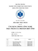
Cost optimal PRAM algorithm complexity:
O(logn) (using n div 2 processors)



Example for n=8 and p=4 processors
a0

j=0

P0

j=1

P0

j=2

P0

a1

a2

P1

a3

a4

a5

P2

a6

a7

P3

P2

Khoa Công Nghệ Thông Tin – Đại Học Bách Khoa Tp.HCM

-6-


Cost Optimal PRAM Algorithm for
the Reduction Problem(cont’d)

Using p= n div 2 processors to add n numbers:

Global a[0..n-1], n, i, j, p;
Begin
spawn(P0, P1,… ,,Pp-1);
for all Pi where 0 ≤ i ≤ p-1 do
for j=0 to ceiling(logp)-1 do
if i mod 2j =0 and 2i + 2j < n then
a[2i] := a[2i]  a[2i + 2j];
endif;
endfor j;
endforall;
End.

Notes: the processors communicate in a biominal-tree pattern
Khoa Công Nghệ Thông Tin – Đại Học Bách Khoa Tp.HCM

-7-


Solving Reducing Problem on
Hypercube SIMD Computer

P6

P4

P0

P0

P2
P7

P5

P1

P2

P0

P3

P1

P1
P3

Step 1:

Step 2:

Step 3:

Reduce by dimension j=2

Reduce by dimension j=1

Reduce by dimension j=0

The total sum will be at P0

Khoa Công Nghệ Thông Tin – Đại Học Bách Khoa Tp.HCM

-8-


Solving Reducing Problem on
Hypercube SIMD Computer (cond’t)

Allocate
workload for
each
processors

Using p processors to add n numbers ( p << n)
Global j;
Local local.set.size, local.value[1..n div p +1], sum,
tmp;
Begin
spawn(P0, P1,… ,,Pp-1);
for all Pi where 0 ≤ i ≤ p-1 do
if (i < n mod p) then local.set.size:= n div p + 1
else local.set.size := n div p;
endif;
sum[i]:=0;
endforall;

Khoa Công Nghệ Thông Tin – Đại Học Baùch Khoa Tp.HCM

-9-


Solving Reducing Problem on
Hypercube SIMD Computer (cond’t)

Calculate the
partial sum for
each processor

for j:=1 to (n div p +1) do
for all Pi where 0 ≤ i ≤ p-1 do
if local.set.size ≥ j then

sum[i]:= sum  local.value [j];

endforall;
endfor j;

Khoa Công Nghệ Thông Tin – Đại Học Bách Khoa Tp.HCM

-10-


Solving Reducing Problem on
Hypercube SIMD Computer (cond’t)

Calculate the total
sum by reducing
for each

dimension of the
hypercube

for j:=ceiling(logp)-1 downto 0 do
for all Pi where 0 ≤ i ≤ p-1 do
if i < 2j then
tmp := [i + 2j]sum;
sum := sum  tmp;
endif;
endforall;
endfor j;

Khoa Công Nghệ Thông Tin – Đại Học Bách Khoa Tp.HCM

-11-


Solving Reducing Problem on
2D-Mesh SIMD Computer



A 2D-mesh with p*p processors need at least 2(p-1) steps to
send data between two farthest nodes
The lower bound of the complexity of any reduction sum
algorithm is 0(n/p2 + p)

Example: a 4*4 mesh
need 2*3 steps to get
the subtotals from the

corner processors

Khoa Công Nghệ Thông Tin – Đại Học Bách Khoa Tp.HCM

-12-


Solving Reducing Problem on
2D-Mesh SIMD Computer(cont’d)


Example: compute the total sum on a 4*4 mesh

Stage 1

Stage 1

Stage 1

Step i = 3

Step i = 2

Step i = 1

Khoa Công Nghệ Thông Tin – Đại Học Bách Khoa Tp.HCM

-13-

Solving Reducing Problem on
2D-Mesh SIMD Computer(cont’d)


Example: compute the total sum on a 4*4 mesh

Stage 2

Stage 2

Stage 2

Step i = 3

Step i = 2

Step i = 1
(the sum is at P1,1)

Khoa Công Nghệ Thông Tin – Đại Học Bách Khoa Tp.HCM

-14-


Solving Reducing Problem on
2D-Mesh SIMD Computer(cont’d)

Stage 1:
Pi,1 computes
the sum of all

processors in
row i-th

Summation (2D-mesh SIMD with l*l processors
Global i;
Local tmp, sum;
Begin
{Each processor finds sum of its local value 
code not shown}
for i:=l-1 downto 1 do
for all Pj,i where 1 ≤ i ≤ l do
{Processing elements in colum i active}
tmp := right(sum);
sum:= sum  tmp;
end forall;
endfor;

Khoa Công Nghệ Thông Tin – Đại Học Bách Khoa Tp.HCM

-15-


Solving Reducing Problem on
2D-Mesh SIMD Computer(cont’d)
Stage2:
Compute the
total sum and
store it at P1,1

for i:= l-1 downto 1 do

for all Pi,1 do
{Only a single processing element active}
tmp:=down(sum);
sum:=sum  tmp;
end forall;
endfor;
End.

Khoa Công Nghệ Thông Tin – Đại Học Bách Khoa Tp.HCM

-16-


Solving Reducing Problem on
UMA Multiprocessor Model(MIMD)




Easily to access data like PRAM
Processors execute asynchronously, so we must ensure
that no processor access an “unstable” variable
Variables used:
Global

a[0..n-1],

{values to be added}

p,

{number of proeessor, a power of 2}

flags[0..p-1],

{Set to 1 when partial sum available}

partial[0..p-1],

{Contains partial sum}

global_sum;

{Result stored here}

Local local_sum;

Khoa Công Nghệ Thông Tin – Đại Học Bách Khoa Tp.HCM

-17-


Solving Reducing Problem on
UMA Multiprocessor Model(cont’d)


Example for UMA multiprocessor with p=8 processors
Stage 2

P0

P1

P2

P3

P4

P5

P6

P7

Step j=8

Step j=4

Step j=2
Step j=1

The total sum is at P0
Khoa Công Nghệ Thông Tin – Đại Học Bách Khoa Tp.HCM

-18-


Solving Reducing Problem on UMA
Multiprocessor Model(cont’d)

Stage 1:
Each processor
computes the
partial sum of n/p
values

Summation (UMA multiprocessor model)
Begin
for k:=0 to p-1 do flags[k]:=0;
for all Pi where 0 ≤ i < p do
local_sum :=0;
for j:=i to n-1 step p do
local_sum:=local_sum  a[j];

Khoa Công Nghệ Thông Tin – Đại Học Bách Khoa Tp.HCM

-19-


Solving Reducing Problem on UMA
Multiprocessor Model(cont’d)
j:=p;
while j>0 do begin

Stage 2:
Compute the total sum

Each processor
waits for the partial

sum of its partner
available

if i ≥ j/2 then
partial[i]:=local_sum;
flags[i]:=1;
break;
else
while (flags[i+j/2]=0) do;
local_sum:=local_sum  partial[i+j/2];
endif;
j=j/2;
end while;
if i=0 then global_sum:=local_sum;
end forall;
End.

Khoa Công Nghệ Thông Tin – Đại Học Baùch Khoa Tp.HCM

-20-