Quantitative NMR Spectroscopy
Bạn đang xem bản rút gọn của tài liệu. Xem và tải ngay bản đầy đủ của tài liệu tại đây (617.36 KB, 8 trang )
Quantitative NMR Spectroscopy.docx 11/2017
Quantitative NMR Spectroscopy
1. Introduction
These notes summarise procedures for the acquisition and processing of quantitative 1H, 19F, 31P, and
13
C NMR data. It is important to note that quantitative NMR (now referred to commonly as qNMR) is
not simply a matter of collecting a 1D spectrum and comparing the integrals. A number of
parameters must be optimised in order to obtain accurate and precise quantitative results.
There are essentially two types of quantitative NMR:
1. Relative concentration determination
For relative concentration determination, you are comparing integrals of interest with one
another. This will allow you to measure accurate ratios of the different species, if not the
actual concentrations themselves.
2. Absolute concentration determination
For absolute concentration determination, you are comparing the integrals of interest to a
known concentration standard, and deriving from these absolute values of concentration,
yield and purity. The concentration standard will be referred to as the calibration compound
or calibrant, to distinguish it from a reference compound, which may be employed for
chemical shift referencing.
2. Relative concentration determination
Relative concentration determination is the most common type of quantitative NMR experiment in
organic chemistry, and the easiest to set up. This method will give you the ratios of compounds in a
mixture. Typical applications include purity evaluation, and isomer ratio determination.
When preparing your sample, ensure that your compound is soluble in the solvent selected, the
concentration is high enough to give good S/N, and that the sample volume is appropriate for NMR.
No calibrant is required.
3. Absolute concentration determination
For absolute concentration determination, in addition to the points above concerning sample
preparation, your sample should contain a known amount of a calibration compound. All
compounds should be weighed as accurately as possible. The calibrant does not need to be
structurally related to the analyte of interest, but it does need to contain the nucleus of interest and
to have resonances that do not overlap with those of the analyte. It is also beneficial if the calibrant
produces relatively simple NMR spectra, with only singlet resonances. Additional requirements for
calibration compounds are that they should be chemically inert, highly soluble in the solvent used,
have low volatility, and not have excessively long T1 relaxation times. It is also beneficial if the
1
Quantitative NMR Spectroscopy.docx 11/2017
calibrant exists in pure form and is easily weighable. Several common 1H quantitative NMR
calibration compounds have been proposed, and some of the more popular examples are found in
Table 1; further examples can be found at />Please speak to a member of the NMR staff if you require help in selecting an appropriate
concentration calibration compound.
If there is no suitable choice of calibrant available, or if sample preparation is an issue, it may be
possible to use an external calibrant. For this, consult a member of the NMR staff.
Solvent solubility
DMSO- CD3OD
d6
Molecular
weight
(g/mol)
116.07
δ
(ppm)
D2O
6.06.3
Fumaric acid
116.07
6.66.8
Sodium acetate
82.03
1.61.9
Dimethyl sulfone
94.13
3.0
TSP-d4
150.29
0.0
1,3,5-trimethoxybenzene
168.19
6.1
3.73.8
1,4-dinitrobenzene
168.11
8.38.5
3,4,5-trichloropyridine
182.43
8.58.8
215.00
-62
(19F)
218.2
-106
(19F)
Calibration Standard
Structure
Maleic acid
2,4Dichlorobenzotrifluoride
4,4’Difluorobenzophenone
1
CDCl3
19
Table 1: Properties of selected H and F calibration standards. Chemical shifts provide a guide but are solvent
dependent within these ranges.
2
Quantitative NMR Spectroscopy.docx 11/2017
4. Signals to be considered for quantification
When analysing a spectrum with multiple peaks, the signal used for quantification should be
unambiguously assigned. In addition, the signal should be as simple as possible, i.e. a singlet is
superior to a multiplet, and have as little overlap as possible with other peaks. Exchangeable
protons, such as amides or hydroxyls, should not be used for quantification due to their broadness
and susceptibility to sample conditions. If signal overlap is an issue, it may be possible to address this
by changing the solvent or pH, or through the use of auxiliary shift reagents.
5. Acquisition
5.1 Parameter sets
Specific parameter sets are available on the spectrometers for quantitative experiments.
Please speak to the NMR staff if you require other nuclei to be defined.
The 1H and 19F experiments do not use 13C decoupling by default. This means that when
integrating your peaks (see below) one needs to be consistent in either including or
excluding the one-bond satellites for every peak considered. The optional use of 13C
decoupling removes the satellite peaks and prevents their overlap with other peaks which
may interfere with accurate quantitation; speak with the NMR staff if you think this is
necessary- in most cases it is not required. The 13C and 31P experiments must use inversegated decoupling, thereby preventing signal enhancement through NOEs.
5.2 Shimming
After inserting the sample in the magnet, wait at least five minutes for the sample
temperature to equilibrate. Tune and shim your sample then run an initial 1D spectrum.
Accurate shimming is essential for quantitative NMR, so if the spectrum shows evidence of
poor shimming (i.e. poor resolution, broad or unsymmetrical peaks), then re-do the
shimming. It is advisable to turn spinning off to prevent artefacts known as “spinning
sidebands”. If poor shimming is still observed after multiple attempts, remove your sample
from the magnet and check that the sample volume is acceptable, the sample is properly
mixed and that the tube is clean.
5.3 Relaxation delay
It is crucial to ensure that all signals have relaxed fully between pulses. Use a relaxation
delay (“d1”) of at least five times the T1 of the slowest relaxing signal of interest in the
spectrum. A major problem here is that the relaxation times of the nuclei in the sample are
often not known, although they can be quickly estimated with an inversion recovery
experiment. T1 values for 1H nuclei in medium-sized molecules typically range from 0.5 to 4
seconds, while those for 13C can range from 0.1 to tens of seconds for quaternary carbons.
For very long 13C relaxation times, it may be necessary to add a relaxation agent.
3
Quantitative NMR Spectroscopy.docx 11/2017
As an example, for a quantitative proton experiment, if the longest 1H T1 in the sample is 4
seconds, the recycle time should be set to at least 20s. In practice, however, the recycle time
is the sum of the relaxation time and the acquisition time. So if the acquisition time is 5s, the
relaxation delay can be set to 15 s, giving 20s in total.
If the relaxation times are not known, the following d1 values are suggested:
1
H: 30s
F: 30s
31
P: 30s
13
C: 60s
19
5.4 Spectral window
There should be sufficient “empty” space on either side of the spectrum so as to ensure that
signals of interest are not affected by attenuation due to receiver filters. A large spectral
width also helps with baseline correction. As a rule of thumb, the spectral width should be
set so that the ends of the spectrum extend by approximately 10% “empty” space on each
side.
5.5 Digital resolution
For accurate integration, each peak should be described by a minimum of four data points
covering the linewidth, and preferably many more. The digital resolution (the spacing
between data points) is defined by the spectral width (“SW”) divided by half the number of
acquired points (“TD”), which also equates to the inverse of the acquisition time (1/AQ). For
a line-width of 1 Hz, which is typical for small to medium-sized molecules, the minimum
digital resolution should therefore be 0.2 Hz, corresponding to an acquisition time of 5s.
The digital resolution in your spectrum can be determined using the command “fidres”.
Having previously defined an appropriate spectral width, the digital resolution should then
be set to at least sw / (td/2) Hz using the parameter “td”.
5.6 Signal to noise
Good signal to noise is essential for accurate integration. For integration errors < 1%, a S/N
of at least 250:1 is required. The number of scans should therefore be set so as to ensure a
good S/N. This will depend on the concentration of your sample. In order to calculate the
signal to noise ratio in your spectrum, use the “sino” command in topspin.
5.7 Excitation bandwidth
The uniform excitation of resonances is also an essential requirement for qNMR. For 1H
spectroscopy this is readily achieved using standard parameters, but for nuclei displaying
greater chemical shift dispersion some caution is required. This is a particular problem for 19F
4
Quantitative NMR Spectroscopy.docx 11/2017
NMR due to its high frequency and larger chemical shift range, but can also be problematic
for 13C NMR. In such cases, it is advisable to compare resonances that have similar chemical
shifts (and to choose calibrants that will enable this) and to place the centre of the spectrum
(defining the transmitter excitation frequency “O1P”) at the midpoint of the peaks to be
compared. Alternative sequences employing excitation with frequency-swept adiabatic
pulses may provide better results; speak to the NMR staff for assistance.
6. Processing
6.1 Zero filling
Ensure that you use zero filling, as this will result in increased integral precision. In order to
use zero filling it is necessary to set the size of the real spectrum (“SI”) to be a multiple of the
number of data points used (“TD”). Setting SI = TD is the minimum amount of zero filling,
and is usually sufficient.
6.2 Line broadening
It is advisable to use line broadening, particularly if the spectrum has low S/N. Normally an
exponential weighting function is used. This is controlled by the parameter “LB”, which by
default is set to 0.3 Hz for 1H and 19F, and 1 Hz for 13C.
Increasing the line broadening will increase the S/N, but decrease the resolution. Conversely,
decreasing the line broadening will increase the resolution at the expense of the S/N. Values
between 0.2 to 1 Hz are typical for 1H and 19F spectra. Higher values are used for 13C spectra,
usually in the range 1 – 5 Hz. Therefore, if increased resolution or S/N is needed, it may be
possible to achieve this by changing the line broadening.
6.3 Accurate phasing
The spectra are phased automatically (eg. The Bruker “apk” command). However, the
phasing should be checked to make sure that it is optimal (see figure 1). If not, the phasing
should be altered manually.
6.4 Baseline correction
A flat baseline is important for accurate integration. The baseline is corrected automatically
once the spectrum is completed (the Bruker “abs n” command). However, the baseline
should be checked manually, and if necessary corrected (see figure 1).
6.5 Define appropriate integration regions.
In order to cover 99 % of the peak area, the integration region should cover at least 20 times
the line width in each direction (figure 2). The integral limits can be decreased if signal
overlap is an issue, however it is important to use the same integral limits for all peaks. For
example, if a peak integral is measured to +/- 50 Hz on each side, all other peaks must also
5
Quantitative NMR Spectroscopy.docx 11/2017
be measured to +/- 50 Hz. In addition, if 13C satellites or spinning sidebands are included in
the integral region for one peak, they should be included for all other peaks measured. If
signal overlap is too severe to allow appropriate integration regions, peak deconvolution can
be used (for example in mestreNova).
Poor baseline!
Poor phasing!
Figure 1: Examples of poor phasing and poor baseline.
Line-width = 0.67 Hz
Integral limits = 20 x line-width
(+/- 0.027 ppm at 500 MHz)
Figure 2: Peak integration- the integrated region should include at least +/- 20x peak half-height
linewidth (Hz).
6
Quantitative NMR Spectroscopy.docx 11/2017
7. Analysis
7.1 Relative concentration determination
Essentially you need to integrate the signals of interest, normalise for the number of protons, and
perform a simple ratio analysis. The molar ratio Mx/My between two compounds x and y can be
determined using the formula:
𝑀𝑥 𝐼𝑥 𝑁𝑦
= ∙
𝑀𝑦 𝐼𝑦 𝑁𝑥
where I is the integral, and N is the number of nuclei giving rise to the signal.
7.2 Absolute concentration determination
This analysis can yield the concentration of the analyte or can directly provide a measure of its
purity.
7.2.1 Molar concentration
The signal(s) corresponding to the calibration compounds must be integrated and normalised
according to the number of protons giving rise to the signal. The integrals of the compound(s) of
interest must then be compared with those of the calibration compound. The concentration of a
compound x in the presence of a calibrant can be calculated using the following formula:
𝐶x =
𝐼x 𝑁cal
×
× 𝐶cal
𝐼cal 𝑁x
where I, N, and C are the integral area, number of nuclei, and concentration of the compound of
interest (x) and the calibrant (cal), respectively. This assumes that the purity of the calibration
compound is 100%. If the purity of the calibrant is not known, it may be useful to do a purity analysis
first.
7.2.2 Purity / yield determination
The purity of a compound x, as a percentage of its nominal weight, can be determined using the
following formula:
𝑃𝑥 =
𝐼𝑥
𝑁𝑐𝑎𝑙
𝑀𝑥
𝑊𝑐𝑎𝑙
×
×
×
× 𝑃𝑐𝑎𝑙
𝐼𝑐𝑎𝑙
𝑁𝑥
𝑀𝑐𝑎𝑙
𝑊𝑥
where, I, N, M, W and P are the integrated area, number of nuclei, molecular mass, gravimetric
weight and purity of the compound of interest (x) and the calibration compound (cal), respectively.
Because this is a weight-based % purity, it allows you to evaluate the purity even if other
components in the sample are invisible by NMR.
7
Quantitative NMR Spectroscopy.docx 11/2017
As an example, figure 3 illustrates a purity determination of a commercial sample of the amino acid
alanine. A nominal mass of 1.78 mg alanine was tested, using 1.2 mg DSS (purity = 98%) as an
internal calibration standard.
Alanine
CH
Alanine
CH3
L-Alanine
DSS
3x(CH3)
13.41
40.24
10.00
Compounds
Alanine: Mx = 89.09 g/mol, W = 3.56 mg. Nominal mass = 1.78 mg.
DSS:
Mcal = 196.34 g/mol, W cal = 0.64 mg, Pcal = 98%
Integrals
Alanine: Ix = 53.65 (Sum of C-H and CH3 proton signals), Nx = 4
DSS:
Ical = 10, Ncal = 9
Purity Evaluation
Px = 96.5%
The commercial sample of alanine is therefore 96.5% pure, meaning that the actual mass of
1
Figure
3: Example
purityisevaluation
alanine
in the of
sample
1.72 mg. using quantitative H NMR.
Nader Amin & Tim Claridge 2017
8