study of through-thickness residual stress by numerical and experimental techniques
Bạn đang xem bản rút gọn của tài liệu. Xem và tải ngay bản đầy đủ của tài liệu tại đây (646.17 KB, 11 trang )
449
Study of through-thickness residual stress by
numerical and experimental techniques
S Rasouli Yazdi, D Retraint and JLu
Lasmis (Mechanical Systems and Concurrent Engineering Laboratory) Troyes, France
Abstract: The quenching process of aluminium alloys is modelled using the finite element method. The
study of residual stress field induced by quenching is divided into two: the thermal and mechanical aspects.
In the thermal problem, the general heat conduction equation is solved and the temperature field during
quenching is calculated. In the mechanical problem, the calculated temperature field and mechanical proper-
ties are used to predict the residual stress field.
In this paper, the two different boundary conditions used in the thermal problem are examined. The first is
surface convection using the appropriate heat transfer coefficient. The second is the temperature variation
measured at the surface of the part. These boundary conditions are compared, and the advantages and the
drawbacks of each are shown.
The influence of different quenching parameters on the level of residual stress is studied. To validate the
quenching modelling, the incremental hole drilling and neutron diffraction methods are used to measure the
residual stress field in the studied parts. The hole drilling technique has been adapted to measure the residual
stress through a larger thickness of the part. The aim of this paper is the combination of numerical and
experimental techniques for the investigation of the through-thickness residual stress field.
Keywords: residual stress, quenching, neutron diffraction, incremental hole drilling, aluminium
NOTATION
A surface area of specimen (m
2
)
A
sn
, B
sn
calibration coefficients for geometry n and
layer s
b plate thickness (m)
C
is
constants at layer s with i ¼ 1; :::; 5
C
p
specific heat capacity (J/kg ЊC)
d
i
, d
0
interreticular spacing of the diffracting planes (m)
e internal energy (J)
˙
e time derivative of internal energy (J/s)
E Young’s modulus (MPa)
h heat transfer coefficient (W/m
2
ЊC)
k conductivity matrix (W/m ЊC)
K coefficient of the Ramberg–Osgood law (MPa)
m mass (kg)
p number of time steps
q heat flux (W/m
2
)
r coefficient of the Ramberg–Osgood law
t time (s)
Dt time interval (s)
T temperature (ЊC)
T
0
fluid temperature (ЊC)
x position from the centre of the plate (m)
a angle between the gauge and the principal
direction 1 (deg)
d
ij
Kronecker delta
strain component
p
plastic strain
r
radial strain
d
el
ij
elastic strain increment related to the stress
increment by Hooke’s law
d
p
ij
plastic strain increment
d
t
ij
total strain increment
d
Th
thermal strain related to the temperature incre-
ment by the thermal expansion coefficient
v
1
, v
0
Bragg angle (deg)
l monochromaticwavelengthofincidentneutrons(m)
n Poisson’s ratio
r density (kg/m
3
)
j stress component (MPa)
j
el
yield stress (MPa)
j
1K
, j
2K
principal stresses (MPa)
j
r
, j
t
radial and tangential stresses respectively (MPa)
t
rt
shearing stress (MPa)
Subscripts
BC boundary condition
E experimental
S00598 ᭧ IMechE 1998 JOURNAL OF STRAIN ANALYSIS VOL 33 NO 6
The MS was received on 11 February 1998 and was accepted after revision
for publication on 1 October 1998.
i normal orientation along the i direction
j principal directions 1, 2 or 3
n time interval number
s layer number
0 quantities measured in the stress-free material
Superscripts
a ambient
TC thermocouple position
1 INTRODUCTION
Heat treatments can improve the mechanical properties of
different alloys. The general heat treatment for aluminium
alloys is quenching with different quenchants such as air,
water and polymer solutions. Each of these quenchants
has a different cooling rate. If the cooling rate is rapid, the
mechanical properties obtained are very interesting but the
level of residual stress and distortion can be great. For a
slow cooling rate, the levels of residual stress and distortion
are lower but the mechanical properties obtained may not be
very useful. Problems with quench distortion, distortion
induced by machining, and residual stress are common, affect-
ing castings, forged products, extrusions and rolled plates. The
residual stress does not always have harmful effects as it is
known a compressive residual stress can improve fatigue
life [1]. Therefore it would be interesting to optimize all
the quenching conditions to obtain the best mechanical
properties, the least distortion and the best fatigue life.
Fatigue life prediction can be deduced from the residual
stress field, but the residual stress level is modified by cyclic
loads [2]. To predict the exact fatigue life, it is necessary to
know the stabilized level of residual stress. Figure 1 shows
the flow diagram for integrating the residual stress in a fati-
gue life prediction. This study can be divided into three:
residual stress field calculation or measurement, residual
stress relaxation and fatigue life calculation.
The fatigue relaxation of residual stress due to quenching
in aluminium alloy 7075 is shown in Fig. 2 [3]. The relaxa-
tion has been modelled using finite element methods. As
shown, the relaxation level depends on the level of applied
loading. The studied alloy is a cyclic hardening material in
which, after a few cycles, the residual stress level was stabi-
lized. A three-dimensional program has been developed in
order to calculate the fatigue life of different parts with dif-
ferent types of applied loading and consideration of the resi-
dual stress [4].
In this paper the first part of the global study is developed.
The residual stress induced by quenching is studied. This
process is modelled by numerical methods using less com-
plex boundary conditions. The residual stress field in the
quenched part has been measured by the modified incremen-
tal hole drilling method and the neutron diffraction method.
The modified hole drilling method has been used because it
gives rapid results. The neutron diffraction method is the
only technique by which to obtain the complete residual
stress field. However, globally as in the future the measured
or calculated residual stress will be integrated in the fatigue
life calculation, measuring the compressive residual stress
in the critical zone near the surface will be sufficient.
2 NUMERICAL MODEL DESCRIPTION
The thermal and mechanical problems are considered as
uncoupled during modelling in the sense that (a) the internal
energy depends on only the temperature and (b) the heat flux
S00598 ᭧ IMechE 1998JOURNAL OF STRAIN ANALYSIS VOL 33 NO 6
Fig. 1 Residual stress integration in the fatigue life calculation
450 S RASOULI YAZDI, D RETRAINT AND J LU
per unit area of the body, flowing into the body, and the heat
supplied externally to the body per unit volume do not
depend on the strains or displacements of the body. In
heat-treatable aluminium alloys, precipitation hardening
during quenching does not induce changes in volume.
Figure 3 shows the necessary procedure for residual stress
prediction. The physical and mechanical data obtained
from the literature are included in the program.
2.1 Temperature field calculation
As the thermal and mechanical problems are not coupled,
the equation of energy conservation is as follows [5]:
¹r
˙
e ¹ div q ¼ 0 ð1Þ
Heat conduction is assumed to be governed by Fourier’s law
[6]:
q ¼ k: grad T ð2Þ
The conductivity can be fully anisotropic, orthotropic or iso-
tropic. In the present case the conductivity is considered as
isotropic; therefore the matrix k is reduced to the scalar k.
Equation (1) together with Fourier’s law [equation (2)]
give the general equation of heat [7]:
rC
p
∂T
∂t
¼ div½k gradðTÞÿ ð3Þ
To obtain the temperature field during quenching, the
general heat equation is solved by numerical methods.
For the time integration, the backward-difference algo-
rithm is used. The non-linear system obtained is solved by
a modified Newton method [8].
2.1.1 Boundary conditions
In the case of quenching at the part surface there is heat
transfer between the part and the quenchant. To define
this heat transfer, boundary conditions must be known.
For the temperature field calculation, the boundary condi-
tions may be specified as the prescribed temperature
T ¼ Tðx; tÞ, the prescribed surface heat flux per area, the
prescribed volumetric heat flux per volume and surface
convection q ¼ hðT ¹ T
0
Þ.
The heat transfer coefficient h depends on the geometry,
quenchant, quenching temperature and material. This para-
meter cannot be determined by pure numerical methods. It
is determined by experimental measurement of tempera-
tures at different points in the quenched material. After
the inverse resolution of the heat transfer conduction equa-
tion for one dimension, using the measured temperatures,
the expression for the heat transfer coefficient is [9, 10]:
h ¼
mC
p
p DtA
ln
T
a
¹ðT
TC
n
Þ
E
T
a
¹ðT
TC
nþp
Þ
E
!
ð4Þ
In equation (4), the time and the position appear, although
S00598 ᭧ IMechE 1998 JOURNAL OF STRAIN ANALYSIS VOL 33 NO 6
Fig. 2 Residual stress relaxation in a quenched cylinder
Fig. 3 Modelling diagram
451STUDY OF RESIDUAL STRESS BY NUMERICAL AND EXPERIMENTAL TECHNIQUES
the heat transfer coefficient does not depend directly on the
time and the position. The coefficient h depends on the tem-
perature; as the temperature depends on the time and the
position, therefore h depends on them too. This boundary
condition requires temperature measurement at different
points of the sample and complex calculations.
Another possible boundary condition is the prescribed
temperature T ¼ Tðx; tÞ. The best solution is to measure
the temperature variation during quenching using thermo-
couples, but measuring the temperature at the surface is
very difficult. Generally it is preferable to measure the sub-
surface temperature. However, applying this measured tem-
perature as a boundary condition does not represent reality
since it is not the exact temperature variation at the part sur-
face. Although in the case of quenching of aluminium
alloys, the heat transfer coefficient and the heat conductivity
are very high, the temperatures at the surface or at a slight
distance from the surface are not very different. Later in
the work these two boundary conditions are applied sepa-
rately and the results obtained are compared.
There is a way to find out the exact temperature variation
at the surface of the part. This consists in measuring the tem-
perature at other points of the part and by extrapolation
obtaining the temperature variation at the part surface. All
these methods introduce errors into the final results. It is
necessary to mention that none of the numerical methods
is 100 per cent accurate.
To obtain the temperature variation, accurate measure-
ment is needed but, to obtain the heat transfer coefficient,
both temperature measurement and complex calculations are
needed. Using surface temperature variation as a boundary
condition is easier because its determination is less complex.
2.2 Thermal results
During quenching there are three phenomena. First, a thin
film of vapour is formed at the surface of the part. During
this time the heat transfer between the part and the quench-
ant is very low; therefore the temperature variation is not
very rapid and the heat transfer coefficient is quite low. Sec-
ond, this film starts to disappear and the heat transfer
increases. At this stage the temperature variation is very
fast and the heat transfer coefficient very high. Third, the
temperature difference between the quenchant and the part
is less; thus the heat transfer decreases, resulting in a low
temperature and variation in heat transfer.
The studied parts are an aluminium alloy 7075 cylinder of
50 mm diameter, an aluminium alloy 7075 plate (500 mm
(length) × 500 mm (width) × 70 mm (height)) and an alumi-
nium alloy 7175 plate (126mm (length) × 53 mm (width) ×
24 mm (height)). Considering the dimensions of the parts,
they can be considered as infinite. Therefore, in the case
of the plates, the heat flow is just through the thickness
and, in the case of the cylinder, it is through the radius.
Figure 4 shows the geometry and the heat flow direction
in the parts. The initial temperature of the parts was
467 ЊC. The aluminium alloy 7075 parts were quenched in
cold water (20 ЊC) and the aluminium alloy 7175 part was
quenched in water at 65 ЊC.
Figure 5 shows the heat transfer coefficient as a function
of time in the first plate (thickness, 70 mm). The three stages
explained before are evident. To calculate the heat transfer
coefficient, thermocouples are used. Four are placed in the
plate thickness as follows: at x ¼ 0mm, x ¼ 17:5 mm,
x ¼ 26mm and x ¼ 34mm where x is the position from
the centre plate. The measured temperatures allow the cal-
culation of the heat transfer coefficient by inverse resolution
of the heat conduction equation.
Figure 6 shows the measured temperatures at four points
in the plate of thickness 70 mm. In the same figure the cal-
culated temperature by extrapolation at the part surface is
shown. The extrapolated temperature at the part surface
S00598 ᭧ IMechE 1998JOURNAL OF STRAIN ANALYSIS VOL 33 NO 6
Fig. 4 Geometry and measurement directions in the parts studied
452 S RASOULI YAZDI, D RETRAINT AND J LU
is obviously not different from the temperature measured
1 mm below the surface.
Two different boundary conditions are applied sepa-
rately: the first is the heat transfer coefficient and the second
is the surface temperature variation during quenching. The
heat transfer coefficient is obtained as explained before
and the surface temperature variation is measured accurately
at the part surface. Figure 7 shows the temperature variation
calculated at the centre of the plate of aluminium alloy 7075
using these two boundary conditions. The results obtained by
each boundary condition are similar. They have been compared
with the measured temperature at the plate centre. Using mea-
sured surface temperature variation is less complex than the
heat transfer calculation; therefore it is more interesting to
use the surface temperature variation as the boundary condition.
2.3 Residual stress field calculation
The temperature field in the first calculation is recorded and
used in the second calculation. The geometry and meshing
are the same as in the first calculation. The procedure used
in the finite element program is based on an incremental
approach. This means that the total strain consists of elastic,
plastic and thermal strains. The basic equation to be used is
[11]
d
t
ij
¼ d
el
ij
þ d
p
ij
þ d
ij
d
Th
ð5Þ
The total strain is strictly a function of geometry and it must
satisfy compatibility. The material is considered isotropic;
therefore the plastic calculations are based on the classic
plasticity theory (the von Mises criterion).
The hardening law is a non-linear isotropic hardening law
which means that the yield stress varies as a function of the
plastic strain:
j ¼ j
el
þ Kð
p
Þ
r
ð6Þ
Equation (6) defines the exact curve of stress as the function
of strain. K and r depend on temperature; they are very low
at high temperatures. All the mechanical and physical prop-
erties have been taken from previous literature [12–14].
2.4 Mechanical results
For mechanical analysis, the calculated temperature field is
transferred. The boundary conditions in this part will be of
the geometrical type. The plates and the cylinder explained
above are modelled respectively as two-dimensional and
axisymmetrical parts. Figure 4 shows the directions of
measurement in the plates and in the cylinder.
The residual stress field is calculated as explained before.
The calculated field is compared with the experimental field.
Figures 8 and 9 show the residual stresses in the plate (thick-
ness, 70 mm) and in the cylinder (diameter, 50 mm). In these
two cases the measured residual stress field is obtained by
the layer removal method [15, 16]. The results for the plate
S00598 ᭧ IMechE 1998 JOURNAL OF STRAIN ANALYSIS VOL 33 NO 6
Fig. 5 Variation in the heat transfer coefficient as a function of
time
Fig. 6 Measured temperature variation at different points of the
plate (thickness, 70 mm) quenched in water at 20 ЊC
Fig. 7 Measured and calculated temperatures using two different
boundary conditions (BCs) at the plate centre (thickness,
70 mm)
453STUDY OF RESIDUAL STRESS BY NUMERICAL AND EXPERIMENTAL TECHNIQUES
and cylinder are given for only half the depth because of
symmetry of the parts. The residual stress field obtained
for the plate of aluminium alloy 7175 (thickness, 24 mm)
is developed further.
In the case of the plates the calculated residual stresses
along the X and Y directions are similar and therefore just
one of these stresses is presented. The calculated residual
stress along the Z direction is zero. In the case of the cylin-
der, the residual stresses along the three directions are dif-
ferent.
With regard to the aluminium alloy 7175 plate (thickness,
24 mm) the quenching has been modelled. As mentioned
before, in the case of the infinite plates the residual stresses
induced by quenching are similar along the X and Y
directions (Fig. 10) (for the directions see Fig. 4). In this
plate the residual stress field has been measured by the
incremental large hole drilling method and the neutron
diffraction method. In the next section, the bases of these
two experimental methods have been developed.
3 EXPERIMENTAL RESULTS
3.1 Neutron diffraction method
3.1.1 Principle
Neutron diffraction is a non-destructive technique enabling
the in-depth residual stress to be evaluated, owing to the
penetration of most materials up to a depth z of several cen-
timetres by the neutron beam. The principle of this method
is very similar to the well-known X-ray diffraction techni-
que which is widely used to determine the surface residual
stress.
When a monochromatic neutron beam interacts with a
crystalline material, incident neutrons are subject to diffrac-
tion at the planes of atoms and produce strongly diffracted
beams leaving in directions defined by Bragg’s law [17]:
l ¼ 2d sinv ð7Þ
Assuming that l is constant, the differentiation of Bragg’s
law (7) gives the following relationship:
i
¼
d
i
¹ d
0
d
0
¼¹
1
2
1
tan v
ð2v
i
¹ 2v
0
Þð8Þ
Then, assuming that the principal directions are not very far
from the natural coordinates of the specimen, the strain
components measured by neutron diffraction are converted
to stress by the generalized Hooke’s law:
j
j
¼
E
1 þ n
j
þ
n
1 ¹ 2n
j
j
ð9Þ
3.1.2 Results
Neutron diffraction measurements were carried out in the
S00598 ᭧ IMechE 1998JOURNAL OF STRAIN ANALYSIS VOL 33 NO 6
Fig. 8 Residual stress in the plate (thickness, 70 mm) quenched
in cold water (20 ЊC)
Fig. 9 Axial residual stress in the cylinder (diameter, 50 mm)
quenched in cold water (20ЊC)
Fig. 10 Residual stress in the quenched plate (thickness, 24 mm)
obtained by the neutron diffraction method and the
numerical method
454 S RASOULI YAZDI, D RETRAINT AND J LU
diffractometer of residual stress and texture measurement
(REST) of the Studsvik Neutron Research Laboratory
(NFL) in Sweden. Strain scans were made in the longitudi-
nal, transverse and normal directions (Y, X and Z directions
respectively) across the (24 mm) thickness of the sample.
The (311) reflection of aluminium, with a 2 mm × 2mm ×
20 mm gauge volume, was used for transverse and normal
measurements. For longitudinal measurements, the gauge
height was reduced to 15 mm because of geometric prob-
lems. The stress-free interplanar spacing d
0
was obtained
by studying three small samples cut out of the same speci-
men. Young’s modulus E and Poisson’s ratio n were calcu-
lated for the (113) crystallographic orientation from
aluminium single-crystal constants using the Kro
¨
ner [18]
model. They were 66 GPa and 0.357 respectively.
The residual stress distribution is plotted in Fig. 10. The
mid-plane located at a depth of 12 mm is the symmetry
plane. The longitudinal (Y direction) and transverse (X
direction) stresses reach as high as 80 MPa in the mid-thick-
ness but are slightly lower in magnitude near both surfaces;
they become tensile at around 7mm under each surface. The
normal stress does not fluctuate very much and remains near
to a zero value. To validate the quenching modelling, the
numerical results have been compared with the experimen-
tal results obtained from the neutron diffraction method in
Fig. 10.
3.2 Incremental large hole drilling method
3.2.1 Principle
The classic incremental hole drilling method is semidestruc-
tive [19]. It consists in drilling a small hole (diameter, from
1 to 5 mm) in the sample and at each depth measuring the
strain in the hole plane. The hole diameter is chosen accord-
ing to the part thickness and the residual stress gradient.
Generally the hole can be drilled to a depth of 50 per cent
of the final hole diameter to measure the residual stress dis-
tribution. The greater the hole diameter, the further one can
drill into the part. In the quenching case the residual stress is
distributed over the depth of the whole part, which means
that there is high compressive residual stress at the part sur-
face and a very high tensile residual stress in the centre of
the part; therefore a large drilling diameter is necessary.
The large hole drilling method is carried out in two faces
of the aluminium alloy 7175 plate (thickness, 24 mm).
Using materials equilibrium laws before and after remov-
ing a layer and if just the layer s is considered, the reaction
stresses at the part surface in the zone where gauges are
placed after hole drilling can be obtained from the following
equations:
j
rs
¼
C
1s
ðj
1ks
þ j
2ks
Þ
2
þ
C
2s
ðj
1ks
¹ j
2ks
Þ
2
cos ð2a
s
Þð10Þ
j
ts
C
3s
ðj
1ks
þ j
2ks
Þ
2
¹
C
4s
ðj
1ks
¹ j
2ks
Þ
2
cosð2a
s
Þð11Þ
t
rts
¼ C
5s
sinð2a
s
Þ
j
2ks
¹ j
1ks
2
ð12Þ
where C
1s
, C
2s
, C
3s
, C
4s
and C
5s
are the constants which
depend on the gauge positions, hole diameters, layer s loca-
tions and the total hole depths:
rs
¼
1
E
ðj
rs
¹ n ¬ j
ts
Þð13Þ
Equation (14) is obtained from equations (10) to (13):
rs
ða
s
Þ¼A
sn
ðj
1ks
þ j
2ks
ÞþB
sn
ðj
1ks
¹ j
2ks
Þ cosð2a
s
Þ
ð14Þ
The A
sn
and B
sn
coefficients are called calibration coeffi-
cients and they depend on the geometry of the hole diameter
gauges, the location of layer s and the hole depth.
These coefficients are calculated by numerical methods
based on the finite element method [20]. The radial strains
are measured by gauges; therefore a
s
, j
1ks
and j
2ks
can be
calculated.
3.2.2 Results
In the quenched plate case, the part thickness is about
24 mm. The chosen diameter is about 10 mm. The hole posi-
tion is in the XY plane (Fig. 4) as far as possible from the part
edges because the plate has been obtained from an infinite
plate and, when cutting the original plate, the residual stres-
ses were relaxed near the edges of the obtained part. For the
chosen diameter there is no existing rosette. As is known
each classic rosette is made of three gauges. In this case,
six gauges are placed around the drilled hole at a distance
equal to approximately the hole diameter from the hole cen-
tre. The angle between two gauges is about 45Њ. Each rosette
uses three gauges; thus from these six gauges it is possible to
form different rosettes which are similar by simply changing
the orientation. In this way the strains which relax during
cutting can be measured at more points on the part surface
and the uniformity verified for the residual stresses calcu-
lated from the measured strains at each depth. The part
has been drilled up to 5mm. To obtain more information
about the residual stress level, another hole was drilled at
exactly the same place as the first but on the other part
face (parallel to the XY plane). As regards the hole depth,
it was possible to go deeper but the chosen diameter was
quite large and, the more the part is drilled, the more the
gauge sensitivity decreases and the more difficult it is to
detect the strains. Our chosen hole diameter is larger than
the usual hole diameters. The finite element calculation
method for the calibration coefficients which are required
to obtain the residual stress field from the measured strains
is the technique generally applied for small holes. In the
case studied, we applied the calculation method to a hole
diameter of 10 mm. Figure 11 shows the measured residual
stress using the large incremental hole drilling method
and the neutron diffraction method. The Y and X residual
S00598 ᭧ IMechE 1998 JOURNAL OF STRAIN ANALYSIS VOL 33 NO 6
455STUDY OF RESIDUAL STRESS BY NUMERICAL AND EXPERIMENTAL TECHNIQUES
stresses are obtained; the difference between them is not
very great. With the incremental hole drilling technique,
the normal (Z direction) residual stress cannot be measured
but in the case of our sample geometry this is not important
because the normal residual stress is nearly zero. As was
expected, there is compressive residual stress at the surface
and it is about 70 MPa.
4 INFLUENCE OF THE QUENCH PARAMETERS
ON THE LEVEL OF RESIDUAL STRESS
After the validation of our model, the effects of the quench-
ing parameters were studied. The level of residual stress
changes with different quenching parameters. These para-
meters are generally defined by the quenchant, the quench-
ing temperature and the quenched zones (with controlled
cooling methods in quenching).
The residual stress field due to quenching has never been
integrated in a fatigue life calculation. For a given fatigue
life, it is possible to define the necessary residual stress field
[21]. Thus it can be interesting to change quenching condi-
tions so as to obtain the residual stress field required for
improved fatigue life. Figure 12 shows the influence of
the quenching temperature on the residual stress level. A
low quenching temperature introduces a high residual stress
into the part, and a high quenching temperature introduces a
low residual stress and a lower distortion. Generally the
quenchant and thequenching temperature influencethecool-
ing speed; therefore, to varythe residual stress level, both the
quenchant and the quenching temperature can be varied.
The compressive residual stress is known to increase the
fatigue life. From the fatigue life calculation it is possible to
determine the part of the sample in which the compressive
residual stress is required so as to define the quenched
zone as a function of the fatigue life [21].
5 DISCUSSION
In Fig. 11 the residual stress field obtained by the modified
incremental hole drilling method and the neutron diffraction
method are compared. In this figure the results are shown to
be not very different. The existing difference is not very
great considering the errors introduced by the measurement
techniques. Estimated errors are Ϯ20 MPa for the incremen-
tal hole drilling method and Ϯ10 MPa for the neutron dif-
fraction method. The level of the measured residual
stresses is not very high. Considering the errors of each
method and the level of the measured residual stress, the
results of each method seem to be acceptable. In Fig. 10
the calculated residual stress is compared with the experi-
mental data. The part has been quenched in water at
65 ЊC. Considering the quenching temperature and the plate
thickness (24 mm), the induced residual stress is not very
high. The maximum compressive stress and the maximum
tensile stress obtained by calculation are about 75 and
55 MPa respectively. These maxima are very similar to
experimental values. The only difference between them is
that the calculated value changes sign (compressive to ten-
sile) at a lower depth than the experimental value does. It is
necessary to mention that, the higher the level of the induced
residual stress, the more accurately the residual stress can be
calculated (Figs 8 and 9). This may be due to mechanical
data such as the yield stress, which in the calculation is sup-
posed to be temperature dependent. Yield stress measure-
ments at different temperatures are not very accurate, and
thus errors can be introduced in the calculation. Another
possible source of error is the residual stress measurements.
Globally the maximum tensile and compressive stresses
have been predicted correctly. The differences obtained
between numerical and experimental results are similar to
the differences obtained in the previous studies [22]. For
high residual stress fields even the distribution throughout
the thickness is correct, whereas for low residual stress
S00598 ᭧ IMechE 1998JOURNAL OF STRAIN ANALYSIS VOL 33 NO 6
Fig. 11 Residual stress in the quenched plate (thickness, 24 mm)
obtained by the neutron diffraction method and the incre-
mental large hole drilling method
Fig. 12 Residual stress in the plate (thickness, 70 mm) quenched
in cold (20 ЊC) and hot (80ЊC) water
456 S RASOULI YAZDI, D RETRAINT AND J LU
fields the calculation predicts fewer thickness effects from
the compressive residual stress. As this calculated residual
stress field is required in a fatigue life calculation, a smaller
depth for the compressive residual stress does not create a
problem because the estimated fatigue life will be shorter
than the real value, thus giving greater safety.
6 CONCLUSIONS
In this study, the hybrid approach of numerical and experi-
mental techniques is developed for a residual stress field
study of quenched parts. This is the first procedure in the
global approach for residual stress integration in fatigue
life prediction. Quenching has been modelled using the
finite element method. Both thermal and mechanical data
are necessary for this modelling. The most important
thermal parameter is the heat transfer coefficient which
enables the boundary conditions in the thermal problem to
be defined. This coefficient is obtained from an experi-
mental temperature field. The heat transfer coefficient is
obtained by inverse resolution of the heat conduction equa-
tion. Different numerical methods can be applied to deter-
mine this coefficient but all of them need the experimental
temperature fields. To reduce the difficulty at this point,
instead of using the heat transfer coefficient to define the
boundary conditions, the measured temperature as near as
possible to the part surface has been used. From these two
different boundary conditions the same temperature field
is obtained. Thus, in the case of materials and quenchants
with a high conductivity, the temperature measured exactly
at the part surface can be used as the boundary condition in
the thermal problem. It is true that using this method can
introduce errors into the calculation but these errors are
small and they are less than the errors obtained from heat
transfer coefficient calculation.
The calculated residual stress field has been compared
with the measured residual stress field. The numerical resi-
dual stress field is close to the experimental value; therefore
the quenching model has been validated. Using the same
model, the quenching has been modelled for different
quenching temperatures. The lower the quenching tempera-
ture, the higher is the residual stress obtained.
The measurement techniques used were the neutron dif-
fraction method and the incremental large hole drilling
method. The incremental large hole drilling method is an
extension of the classic incremental hole drilling method.
This technique enables more rapid measurement of the
residual stress at a greater depth to be made. The residual
stress obtained by this method has been compared with
the residual stress field obtained by the neutron diffraction
method. The residual stress levels in these two cases are
close considering the errors due to each technique; therefore
the incremental large hole drilling method can be taken as
valid. With this modified technique it is possible to measure
the through-thickness residual stress field induced by heat
treatments or surface treatments of different types of alloy.
The next stage of this study is to integrate the residual
stress field due to quenching in a fatigue life calculation.
Before this, calculation of the relaxation of residual stress
has to be taken into account.
ACKNOWLEDGEMENTS
The authors are grateful to the Studsvik Neutron Research
Laboratory for their help in the measurement of residual
stress by neutron diffraction method. The authors are also
grateful to Mr G. Houset and Mr A. Voinier at the Univer-
site
´
de Technologie de Troyes for their technical help. The
authors are also grateful to ‘Pole de Mode
´
lisation’ for its
financial support.
REFERENCES
1 Lu, J., Flavenot, J. F. and Lieurade, H. P. Inte
´
gration de la
notion des contraintes re
´
siduelles dans les bureaux d’e
´
tudes,
les contraintes re
´
siduelles au bureau d’e
´
tudes. CETIM, Senlis,
France, 1991, pp. 9–34.
2 Lu, J., Flavenot, J. F. and Turbat, A. Prediction of residual
stress relaxation during fatigue. In Mechanical Relaxation of
Residual Stresses, ASTM special technical publication 993
(Ed. L. Mordfin),1988, pp. 75–90 (American Society for Test-
ing and Materials, Philadelphia, Pennsylvania).
3 Rasouli Yazdi, S. and Lu, J. Simulation of quenching and
fatigue relaxation of residual stresses in aluminum parts. In
Proceedings of the Fifth International Conference on Residual
Stresses (Eds T. Ericsson, M. Ode
´
n and A. Andersson), Insti-
tute of Technology, Linko
¨
ping Universitet, Linko
¨
ping,
Sweden, 1997, pp. 490–495.
4 Akrache, R. and Lu, J. Fatigue life prediction for 3D struc-
tures. In Proceedings of the Fifth International Conference
on Computational Plasticity (Eds D. R. J. Owen, E. Onate
and E. Hinton), Barcelona, 1997, pp. 1021–1026 (CIMNE,
Barcelona, Spain).
5 Lemaitre, L. and Chaboche, J.L. Me
´
canique des Mate
´
riaux
Solides, 1984 (Dunod, Paris).
6 Landau, L. and Lifchitz, E. Physique The
´
orique, Vol. 6, 2nd
edition, 1989, pp. 273–334 (Mir, Moscow).
7 Fletcher, A. J. Thermal Stress and Strain Generation in Heat
Treatment, 1989 (Elsevier Applied Science, Barking, Essex,
and The Universities Press, Belfast).
8 ABAQUS Theory Manual, 1996 (Hibitt, Karlsson and
Sorensen, Incorporated, USA).
9 Price, R.F. and Fletcher, A. J. Generation of thermal stress
and strain during quenching of low alloy steel plates. Metals
Technol. (Lond.), 1981, 8, 427–446.
10 Fletcher, A. J. and Nasseri, M. Effect of plate orientation on
quenching characteristics. Mater. Sci. Technol., 1995, 11,
375–381.
11 Beck, G. and Ericsson, T. Prediction of Residual Stresses due
to Heat Treatment, 1987, pp. 27–40 (Deutsche Gesellschaft
fu
¨
r Metallkunde Informationsgesellschaft mbH, Oberursel).
12 Hatch, J. E. Aluminum—Properties and Physical Metallurgy,
1984 (American Society for Metals, Metals Park, Ohio).
13 Ledbetter, H. M. Temperature behaviour of Young’s moduli
S00598 ᭧ IMechE 1998 JOURNAL OF STRAIN ANALYSIS VOL 33 NO 6
457STUDY OF RESIDUAL STRESS BY NUMERICAL AND EXPERIMENTAL TECHNIQUES
of forty engineering alloys. In Materials Studies for Magnetic
Fusion Energy Applications at Low Temperature—IV, 1981,
pp. 257–269.
14 Takeuti, Y. G., Komori, S., Noda, N. and Nyuko, H. Ther-
mal stress problems in industry. 3: Temperature dependency
of elastic moduli for several metals at temperatures from
–196 to 1000ЊC. J. Thermal Stresses, 1979, 2, 233–250.
15 Jeanmart, P. H. and Bouvaist, J. Finite element calculation
and measurement of thermal stresses in high strength alumi-
num alloys. In Advances in Surface Treatments Technology
Applications—Effects, Vol. 4, Residual Stresses, 1987, pp.
327–340 (Pergamon, Oxford).
16 Habachou, R. Mode
´
lisation de la trempe et du de
´
tensionne-
ment par de
´
formation plastique des barres et plaques d’al-
liages d’aluminium. The
`
se de doctorat, Institut National des
Sciences Applique
´
es de Lyon, 1983.
17 Holden, T. M. and Roy, G. The application of neutron diffraction
to the measurement of residual stress and strain. In Handbook of
Measurement of Residual Stresses (Ed. J. Lu), 1996, pp. 133–
148 (Society for Experimental Mechanics, New York) (Fairmont
Press and Prentice-Hall, Englewood Cliffs, New Jersey).
18 Kro
¨
ner, E. Berechnung der elastischen Konstanten des Vielk-
ristalls aus den Konstanten des einkristalls. Z. Physik, 1958,
151, 504–505.
19 Schajer, G. S., Roy, G., Flaman, M. T. and Lu, J. Hole dril-
ling and ring core methods. In Handbook of Measurement of
Residual Stresses (Ed. J. Lu) 1996, pp. 5–34 (Society for
Experimental Mechanics, New York) (Fairmont Press and
Prentice-Hall, Englewood Cliffs, New Jersey).
20 Lu, J. De
´
veloppement de la me
´
thode de mesure de contraintes
re
´
siduelles par le perc¸age pas a
`
pas. The
`
se de doctorat, Univer-
site
´
de Technologie de Compie
`
gne, 1986.
21 Akrache, R. Pre
´
vision de la dure
´
e de vie en fatigue des struc-
tures 3D par la me
´
thode des e
´
le
´
ments finis. The
`
se de doctorat,
Universite
´
de Technologie de Compie
`
gne, 1998.
22 Becker, R., Karabin, M. E., Liu, J. C. and Smelser, R. E.
Distortion and residual stress in quenched aluminum bars. J.
Appl. Mechanics,63, 1996, pp. 699–705.
S00598 ᭧ IMechE 1998JOURNAL OF STRAIN ANALYSIS VOL 33 NO 6
458 S RASOULI YAZDI, D RETRAINT AND J LU