mathematics for 3d game programming and computer graphics, third edition [electronic resource]

Mathematics for
3D Game Programming
and Computer Graphics
Third Edition
Eric Lengyel











Course Technology PTR
A part of Cengage Learning







Australia • Brazil • Japan • Korea • Mexico • Singapore • Spain • United Kingdom • United States

Mathematics for 3D Game Programming
and Computer Graphics, Third Edition
By Eric Lengyel

Publisher and General Manager,
Course Technology PTR:
Stacy L. Hiquet

Associate Director of Marketing:
Sarah Panella

Manager of Editorial Services:
Heather Talbot

Marketing Manager:
Jordan Castellani

Senior Acquisitions Editor:
Emi Smith

Cover Designer:
Mike Tanamachi

Proofreader:
Mike Beady

© 2012 Course Technology, a part of Cengage Learning.

ALL RIGHTS RESERVED. No part of this work covered by the copyright
herein may be reproduced, transmitted, stored, or used in any form or by

any means graphic, electronic, or mechanical, including but not limited to
photocopying, recording, scanning, digitizing, taping, Web distribution,
information networks, or information storage and retrieval systems, except
as permitted under Section 107 or 108 of the 1976 United States Copyright
Act, without the prior written permission of the publisher.

For product information and technology assistance, contact us at
Cengage Learning Customer & Sales Support, 1-800-354-9706
For permission to use material from this text or product,
submit all requests online at cengage.com/permissions
Further permissions questions can be emailed to


All trademarks are the property of their respective owners.
All images © Cengage Learning unless otherwise noted.

Library of Congress Control Number: 2011924487
ISBN-13: 978-1-4354-5886-4
ISBN-10: 1-4354-5886-9

Course Technology, a part of Cengage Learning
20 Channel Center Street
Boston, MA 02210
USA

Cengage Learning is a leading provider of customized learning solutions
with office locations around the globe, including Singapore, the United
Kingdom, Australia, Mexico, Brazil, and Japan. Locate your local office at:
international.cengage.com/region

Cengage Learning products are represented in Canada by Nelson
Education, Ltd.

For your lifelong learning solutions, visit courseptr.com
Visit our corporate website at cengage.com


Printed in China
1 2 3 4 5 6 7 13 12 11
eISBN-10: 1-4354-5887-7
 iii


Contents

Preface xiii
What’s New in the Third Edition xiii
Contents Overview xiv
Website and Code Listings xvii
Notational Conventions xvii
Chapter 1 The Rendering Pipeline 1
1.1 Graphics Processors 1
1.2 Vertex Transformation 4
1.3 Rasterization and Fragment Operations 6
Chapter 2 Vectors 11
2.1 Vector Properties 11
2.2 The Dot Product 15
2.3 The Cross Product 19
2.4 Vector Spaces 26
Chapter 2 Summary 29

Exercises for Chapter 2 30
Chapter 3 Matrices 31
3.1 Matrix Properties 31
3.2 Linear Systems 34
3.3 Matrix Inverses 40
3.4 Determinants 47
3.5 Eigenvalues and Eigenvectors 54
3.6 Diagonalization 58
iv Contents

Chapter 3 Summary 62
Exercises for Chapter 3 64
Chapter 4 Transforms 67
4.1 Linear Transformations 67
4.1.1 Orthogonal Matrices 68
4.1.2 Handedness 70
4.2 Scaling Transforms 70
4.3 Rotation Transforms 71
4.3.1 Rotation About an Arbitrary Axis 74
4.4 Homogeneous Coordinates 75
4.4.1 Four-Dimensional Transforms 76
4.4.2 Points and Directions 77
4.4.3 Geometrical Interpretation of the w Coordinate 78
4.5 Transforming Normal Vectors 78
4.6 Quaternions 80
4.6.1 Quaternion Mathematics 80
4.6.2 Rotations with Quaternions 82
4.6.3 Spherical Linear Interpolation 86
Chapter 4 Summary 89
Exercises for Chapter 4 91

Chapter 5 Geometry for 3D Engines 93
5.1 Lines in 3D Space 93
5.1.1 Distance Between a Point and a Line 93
5.1.2 Distance Between Two Lines 94
5.2 Planes in 3D Space 97
5.2.1 Intersection of a Line and a Plane 98
5.2.2 Intersection of Three Planes 99
5.2.3 Transforming Planes 101
5.3 The View Frustum 102
5.3.1 Field of View 103
5.3.2 Frustum Planes 106
5.4 Perspective-Correct Interpolation 107
5.4.1 Depth Interpolation 108
5.4.2 Vertex Attribute Interpolation 110
5.5 Projections 111
5.5.1 Perspective Projections 112
5.5.2 Orthographic Projections 116
 v

5.5.3 Extracting Frustum Planes 118
5.6 Reflections and Oblique Clipping 120
Chapter 5 Summary 126
Exercises for Chapter 5 129
Chapter 6 Ray Tracing 131
6.1 Root Finding 131
6.1.1 Quadratic Polynomials 131
6.1.2 Cubic Polynomials 132
6.1.3 Quartic Polynomials 135
6.1.4 Newton’s Method 136
6.1.5 Refinement of Reciprocals and Square Roots 139

6.2 Surface Intersections 140
6.2.1 Intersection of a Ray and a Triangle 141
6.2.2 Intersection of a Ray and a Box 143
6.2.3 Intersection of a Ray and a Sphere 144
6.2.4 Intersection of a Ray and a Cylinder 145
6.2.5 Intersection of a Ray and a Torus 147
6.3 Normal Vector Calculation 148
6.4 Reflection and Refraction Vectors 149
6.4.1 Reflection Vector Calculation 150
6.4.2 Refraction Vector Calculation 151
Chapter 6 Summary 153
Exercises for Chapter 6 154
Chapter 7 Lighting and Shading 157
7.1 RGB Color 157
7.2 Light Sources 158
7.2.1 Ambient Light 158
7.2.2 Directional Light Sources 159
7.2.3 Point Light Sources 159
7.2.4 Spot Light Sources 160
7.3 Diffuse Reflection 161
7.4 Specular Reflection 162
7.5 Texture Mapping 164
7.5.1 Standard Texture Maps 166
7.5.2 Projective Texture Maps 167
7.5.3 Cube Texture Maps 169
7.5.4 Filtering and Mipmaps 171
vi Contents

7.6 Emission 174
7.7 Shading Models 175

7.7.1 Calculating Normal Vectors 175
7.7.2 Gouraud Shading 176
7.7.3 Blinn-Phong Shading 177
7.8 Bump Mapping 178
7.8.1 Bump Map Construction 178
7.8.2 Tangent Space 180
7.8.3 Calculating Tangent Vectors 180
7.8.4 Implementation 185
7.9 A Physical Reflection Model 187
7.9.1 Bidirectional Reflectance Distribution Functions 187
7.9.2 Cook-Torrance Illumination 191
7.9.3 The Fresnel Factor 192
7.9.4 The Microfacet Distribution Function 195
7.9.5 The Geometrical Attenuation Factor 198
7.9.6 Implementation 200
Chapter 7 Summary 205
Exercises for Chapter 7 209
Chapter 8 Visibility Determination 211
8.1 Bounding Volume Construction 211
8.1.1 Principal Component Analysis 212
8.1.2 Bounding Box Construction 215
8.1.3 Bounding Sphere Construction 217
8.1.4 Bounding Ellipsoid Construction 218
8.1.5 Bounding Cylinder Construction 220
8.2 Bounding Volume Tests 221
8.2.1 Bounding Sphere Test 221
8.2.2 Bounding Ellipsoid Test 222
8.2.3 Bounding Cylinder Test 226
8.2.4 Bounding Box Test 228
8.3 Spatial Partitioning 230

8.3.1 Octrees 230
8.3.2 Binary Space Partitioning Trees 232
8.4 Portal Systems 235
8.4.1 Portal Clipping 236
8.4.2 Reduced View Frustums 238
 vii

Chapter 8 Summary 240
Exercises for Chapter 8 244
Chapter 9 Polygonal Techniques 245
9.1 Depth Value Offset 245
9.1.1 Projection Matrix Modification 246
9.1.2 Offset Value Selection 247
9.1.3 Implementation 248
9.2 Decal Application 249
9.2.1 Decal Mesh Construction 250
9.2.2 Polygon Clipping 252
9.3 Billboarding 254
9.3.1 Unconstrained Quads 254
9.3.2 Constrained Quads 257
9.3.3 Polyboards 258
9.4 Polygon Reduction 260
9.5 T-Junction Elimination 264
9.6 Triangulation 267
Chapter 9 Summary 274
Exercises for Chapter 9 277
Chapter 10 Shadows 279
10.1 Shadow Casting Set 279
10.2 Shadow Mapping 281
10.2.1 Rendering the Shadow Map 281

10.2.2 Rendering the Main Scene 283
10.2.3 Self-Shadowing 284
10.3 Stencil Shadows 286
10.3.1 Algorithm Overview 286
10.3.2 Infinite View Frustums 291
10.3.3 Silhouette Determination 294
10.3.4 Shadow Volume Construction 299
10.3.5 Determining Cap Necessity 303
10.3.6 Rendering Shadow Volumes 307
10.3.7 Scissor Optimization 309
Chapter 10 Summary 314
Exercises for Chapter 10 315
viii Contents

Chapter 11 Curves and Surfaces 317
11.1 Cubic Curves 317
11.2 Hermite Curves 320
11.3 Bézier Curves 322
11.3.1 Cubic Bézier Curves 322
11.3.2 Bézier Curve Truncation 326
11.3.3 The de Casteljau Algorithm 327
11.4 Catmull-Rom Splines 329
11.5 Cubic Splines 331
11.6 B-Splines 334
11.6.1 Uniform B-Splines 335
11.6.2 B-Spline Globalization 340
11.6.3 Nonuniform B-Splines 342
11.6.4 NURBS 345
11.7 Bicubic Surfaces 348
11.8 Curvature and Torsion 350

Chapter 11 Summary 355
Exercises for Chapter 11 357
Chapter 12 Collision Detection 361
12.1 Plane Collisions 361
12.1.1 Collision of a Sphere and a Plane 362
12.1.2 Collision of a Box and a Plane 364
12.1.3 Spatial Partitioning 366
12.2 General Sphere Collisions 366
12.3 Sliding 371
12.4 Collision of Two Spheres 372
Chapter 12 Summary 376
Exercises for Chapter 12 378
Chapter 13 Linear Physics 379
13.1 Position Functions 379
13.2 Second-Order Differential Equations 381
13.2.1 Homogeneous Equations 381
13.2.2 Nonhomogeneous Equations 385
13.2.3 Initial Conditions 388
13.3 Projectile Motion 390
13.4 Resisted Motion 394
 ix

13.5 Friction 396
Chapter 13 Summary 400
Exercises for Chapter 13 402
Chapter 14 Rotational Physics 405
14.1 Rotating Environments 405
14.1.1 Angular Velocity 405
14.1.2 The Centrifugal Force 407
14.1.3 The Coriolis Force 408

14.2 Rigid Body Motion 410
14.2.1 Center of Mass 410
14.2.2 Angular Momentum and Torque 413
14.2.3 The Inertia Tensor 414
14.2.4 Principal Axes of Inertia 422
14.2.5 Transforming the Inertia Tensor 426
14.3 Oscillatory Motion 430
14.3.1 Spring Motion 430
14.3.2 Pendulum Motion 434
Chapter 14 Summary 436
Exercises for Chapter 14 438
Chapter 15 Fluid and Cloth Simulation 443
15.1 Fluid Simulation 443
15.1.1 The Wave Equation 443
15.1.2 Approximating Derivatives 447
15.1.3 Evaluating Surface Displacement 450
15.1.4 Implementation 453
15.2 Cloth Simulation 457
15.2.1 The Spring System 457
15.2.2 External Forces 459
15.2.3 Implementation 459
Chapter 15 Summary 461
Exercises for Chapter 15 462
Chapter 16 Numerical Methods 463
16.1 Trigonometric Functions 463
16.2 Linear Systems 465
16.2.1 Triangular Systems 465
16.2.2 Gaussian Elimination 467
x Contents

16.2.3 LU Decomposition 470
16.2.4 Error Reduction 477
16.2.5 Tridiagonal Systems 479
16.3 Eigenvalues and Eigenvectors 483
16.4 Ordinary Differential Equations 490
16.4.1 Euler’s Method 490
16.4.2 Taylor Series Method 492
16.4.3 Runge-Kutta Method 493
16.4.4 Higher-Order Differential Equations 495
Chapter 16 Summary 496
Exercises for Chapter 16 498
Appendix A Complex Numbers 499
A.1 Definition 499
A.2 Addition and Multiplication 499
A.3 Conjugates and Inverses 500
A.4 The Euler Formula 501
Appendix B Trigonometry Reference 505
B.1 Function Definitions 505
B.2 Symmetry and Phase Shifts 506
B.3 Pythagorean Identities 507
B.4 Exponential Identities 507
B.5 Inverse Functions 508
B.6 Laws of Sines and Cosines 509
Appendix C Coordinate Systems 513
C.1 Cartesian Coordinates 513
C.2 Cylindrical Coordinates 514
C.3 Spherical Coordinates 516
C.4 Generalized Coordinates 520
Appendix D Taylor Series 523
D.1 Derivation 523

D.2 Power Series 525
D.3 The Euler Formula 526
Appendix E Answers to Exercises 529
Chapter 2 529
 xi

Chapter 3 529
Chapter 4 530
Chapter 5 530
Chapter 6 530
Chapter 7 531
Chapter 8 531
Chapter 9 531
Chapter 10 531
Chapter 11 532
Chapter 12 532
Chapter 13 532
Chapter 14 533
Chapter 15 534
Chapter 16 534
Index 535

This page intentionally left blank
 xiii


Preface
This book illustrates mathematical techniques that a software engineer would
need to develop a professional-quality 3D graphics engine. Particular attention is
paid to the derivation of key results in order to provide a complete exposition of

the subject and to encourage a deep understanding of the mechanics behind the
mathematical tools used by game programmers.
Most of the material in this book is presented in a manner that is independent
of the underlying 3D graphics system used to render images. We assume that the
reader is familiar with the basic concepts needed to use a 3D graphics library and
understands how models are constructed out of vertices and polygons. However,
the book begins with a short review of the rendering pipeline as it is implemented
in the OpenGL library. When it becomes necessary to discuss a topic in the con-
text of a 3D graphics library, OpenGL is the one that we choose due to its availa-
bility across multiple platforms.
Each chapter ends with a summary of the important equations and formulas
derived within the text. The summary is intended to serve as a reference tool so
that the reader is not required to wade through long discussions of the subject
matter in order to find a single result. There are also several exercises at the end
of each chapter. The answers to exercises requiring a calculation are given in
Appendix E.
What’s New in the Third Edition
The following list highlights the major changes and additions in the third edition.
Many minor additions and enhancements have also been made, including updates
to almost all of the figures in the book.
■ A discussion of oblique near plane clipping has been added to the view frus-
tum topics covered in Chapter 5.
xiv Preface

■ Chapter 10 now begins with a discussion of shadow casting set determination
before going into discussions of shadow generation techniques.
■ In addition to the stencil shadow algorithm, the shadow mapping technique is
now covered in Chapter 10.
■ The discussion of the inertia tensor in Chapter 14 has been expanded.
■ Chapter 15 has been expanded to include an introduction to cloth simulation

in addition to its discussion of fluid surface simulation.
■ A fast method for calculating the sine and cosine functions has been added to
the beginning of the numerical methods coverage in Chapter 16.
Contents Overview
Chapter 1: The Rendering Pipeline. This is a preliminary chapter that provides
an overview of the rendering pipeline in the context of the OpenGL library.
Many of the topics mentioned in this chapter are examined in higher detail else-
where in the book, so mathematical discussions are intentionally avoided here.
Chapter 2: Vectors. This chapter begins the mathematical portion of the book
with a thorough review of vector quantities and their properties. Vectors are of
fundamental importance in the study of 3D computer graphics, and we make ex-
tensive use of operations such as the dot product and cross product throughout
the book.
Chapter 3: Matrices. An understanding of matrices is another basic necessity of
3D game programming. This chapter discusses elementary concepts such as ma-
trix representation of linear systems as well as more advanced topics, including
eigenvectors and diagonalization, which are required later in the book. For com-
pleteness, this chapter goes into a lot of detail to prove various matrix properties,
but an understanding of those details is not essential when using matrices later in
the book, so the uninterested reader may skip over the proofs.
Chapter 4: Transforms. In Chapter 4, we investigate matrices as a tool for per-
forming transformations such as translations, rotations, and scales. We introduce
the concept of four-dimensional homogeneous coordinates, which are widely
used in 3D graphics systems to move between different coordinate spaces. We
also study the properties of quaternions and their usefulness as a transformation
tool.
ContentsOverview xv

Chapter 5: Geometry for 3D Engines. It is at this point that we begin to see
material presented in the previous three chapters applied to practical applications

in 3D game programming and computer graphics. After analyzing lines and
planes in 3D space, we introduce the view frustum and its relationship to the vir-
tual camera. This chapter includes topics such as field of view, perspective-
correct interpolation, and projection matrices.
Chapter 6: Ray Tracing. Ray tracing methods are useful in many areas of game
programming, including light map generation, line-of-sight determination, and
collision detection. This chapter begins with analytical and numerical root-
finding techniques, and then presents methods for intersecting rays with common
geometrical objects. Finally, calculation of reflection and refraction vectors is
discussed.
Chapter 7: Lighting and Shading. Chapter 7 discusses a wide range of topics
related to illumination and shading methods. We begin with an enumeration of
the different types of light sources and then proceed to simple reflection models.
Later, we inspect methods for adding detail to rendered surfaces using texture
maps, gloss maps, and bump maps. The chapter closes with a detailed explana-
tion of the Cook-Torrance physical illumination model.
Chapter 8: Visibility Determination. The performance of a 3D engine is heavi-
ly dependent on its ability to determine what parts of a scene are visible. This
chapter presents methods for constructing various types of bounding volumes and
subsequently testing their visibility against the view frustum. Large-scale visibil-
ity determination enabled through spatial partitioning and the use of portal sys-
tems is also examined.
Chapter 9: Polygonal Techniques. Chapter 9 presents several techniques in-
volving the manipulation of polygonal models. The first topic covered is decal
application to arbitrary surfaces and includes a related method for performing
vertex depth offset. Other topics include billboarding techniques used for various
special effects, a polygon reduction technique, T-junction elimination, and poly-
gon triangulation.
Chapter 10: Shadows. This chapter discusses shadow-casting sets and the two
prominent methods for generating shadows in a real-time application, shadow

mapping and stencil shadows. The presentation of the stencil shadow algorithm is
particularly detailed because it draws on several smaller geometric techniques.
xvi Preface

Chapter 11: Curves and Surfaces. In this chapter, we examine of a broad varie-
ty of cubic curves, including Bézier curves and B-splines. We also discuss how
concepts pertaining to two-dimensional curves are extended to three-dimensional
surfaces.
Chapter 12: Collision Detection. Collision detection is necessary for interaction
between different objects in a game universe. This chapter presents general
methods for determining whether moving objects collide with the static environ-
ment and whether they collide with each other.
Chapter 13: Linear Physics. At this point in the book, we begin a two-chapter
survey of various topics in classical physics that pertain to the motion that objects
are likely to exhibit in a 3D game. Chapter 13 begins with a discussion of posi-
tion functions as solutions to second-order differential equations. We then inves-
tigate projectile motion both through empty space and through a resistive medi-
um, and close with a look at frictional forces.
Chapter 14: Rotational Physics. Chapter 14 continues the treatment of physics
with a rather advanced exposition on rotation. We first study the forces experi-
enced by an object in a rotating environment. Next, we examine rigid body mo-
tion and derive the relationship between angular velocity and angular momentum
through the inertia tensor. Also included is a discussion of the oscillatory motion
exhibited by springs and pendulums.
Chapter 15: Fluid and Cloth Simulation. We continue with the theme of phys-
ical simulation by presenting a physical model for fluid motion based on the two-
dimensional wave equation and cloth motion based on a spring-damper system.
Chapter 16: Numerical Methods. The book finishes with an examination of
numerical techniques for calculating trigonometric functions and solving three
particular types of problems. We first discuss effective methods for finding the

solutions to linear systems of any size. Next, we present an iterative technique for
determining the eigenvalues and eigenvectors of a
3
3

symmetric matrix. Final-
ly, we study methods for approximating the solutions to ordinary differential
equations.
Appendix A: Complex Numbers.
Although not used extensively, complex
numbers do appear in a few places in the text. Appendix A reviews the concept
of complex numbers and discusses the properties that are used elsewhere in the
book.
WebsiteandCodeListings xvii

Appendix B: Trigonometry Reference. Appendix B reviews the trigonometric
functions and quickly derives many formulas and identities that are used
throughout this book.
Appendix C: Coordinate Systems. Appendix C provides a brief overview of
Cartesian coordinates, cylindrical coordinates, and spherical coordinates. These
coordinate systems appear in several places throughout the book, but are used
most extensively in Chapter 14.
Appendix D: Taylor Series. The Taylor series of various functions are em-
ployed in a number of places throughout the book. Appendix D derives the Tay-
lor series and reviews power series representations for many common functions.
Appendix E: Answers to Exercises. This appendix contains the answer to every
exercise in the book having a solution that can be represented by a mathematical
expression.
Website and Code Listings
The official website for this book can be found at the following address:

All of the code listings in the book can be downloaded from this website. Some
of the listings make use of simple structures such as
Triangle and Edge or
mathematical classes such as
Vector3D and Matrix3D. The source code for
these can also be found on the website.
The language used for all code that is intended to run on the CPU is standard
C++. Vertex shaders and fragment shaders that are intended to run on the GPU
use the OpenGL Shading Language (GLSL).
Notational Conventions
We have been careful to use consistent notation throughout this book. Scalar
quantities are always represented by italic Roman or Greek letters. Vectors, ma-
trices, and quaternions are always represented by bold letters. A single compo-
nent of a vector, matrix, or quaternion is a scalar quantity, so it is italic. For ex-
ample, the
x component of the vector v is written
x
v
. These conventions and other
notational standards used throughout the book are summarized in the table on the
next page.
xviii Preface

Quantity/Operation Notation/Examples
Scalars Italic letters: x, t, A,

,


Angles Italic Greek letters:

,

,


Vectors Boldface letters: V, P, x, ω
Quaternions Boldface letters: q,
1
q
,
2
q

Matrices Boldface letters: M, P
RGB Colors Script letters: , ,

,


Magnitude of a vector Double bar:
P

Conjugate of a complex number z or a
quaternion q
Overbar:
z ,
q

Transpose of a matrix Superscript T:
T
M

Determinant of a matrix det M or single bars:
M

Time derivative
Dot notation:
 
d
tt
dt
xx


Binomial coefficient

!
!!
n
n
k
knk









Floor of x
x





Ceiling of x
x





Fractional part of x


frac
x

Sign of x

1, if 0
sgn 0, if 0
1, if 0
x
x
x

x











Closed interval




,|ab x a x b



Open interval




,|ab x a x b




Interval closed at one end and open at
the other end







,|
,|
ab x a x b
ab x a x b





Set of real numbers 

Set of complex numbers 

Set of quaternions 


 1

Chapter 1
The Rendering Pipeline
This chapter provides a preliminary review of the rendering pipeline. It covers

general functions, such as vertex transformation and primitive rasterization,
which are performed by modern 3D graphics hardware. Readers who are familiar
with these concepts may safely skip ahead. We intentionally avoid mathematical
discussions in this chapter and instead provide pointers to other parts of the book
where each particular portion of the rendering pipeline is examined in greater
detail.
1.1 Graphics Processors
A typical scene that is to be rendered as 3D graphics is composed of many sepa-
rate objects. The geometrical forms of these objects are each represented by a set
of vertices and a particular type of graphics primitive that indicates how the ver-
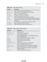
tices are connected to produce a shape. Figure 1.1 illustrates the ten types of
graphics primitive defined by the OpenGL library. Graphics hardware is capable
of rendering a set of individual points, a series of line segments, or a group of
filled polygons. Most of the time, the surface of a 3D model is represented by a
list of triangles, each of which references three points in a list of vertices.
The usual modern 3D graphics board possesses a dedicated Graphics Pro-
cessing Unit (GPU) that executes instructions independently of the Central Pro-
cessing Unit (CPU). The CPU sends rendering commands to the GPU, which
then performs the rendering operations while the CPU continues with other tasks.
This is called asynchronous operation. When geometrical information is submit-
ted to a rendering library such as OpenGL, the function calls used to request the
rendering operations typically return a significant amount of time before the GPU
has finished rendering the graphics. The lag time between the submission of a
rendering command and the completion of the rendering operation does not nor-
mally cause problems, but there are cases when the time at which drawing com-
2 1.TheRenderingPipeline

0
1
2

3
Points
Lines
Triangles
Quads
2
4
5
3
01
2
4
5
3
0
1
2
4
56
7
30
1
Quad Strip
Triangle Strip
Line Strip
2
4
3
0
1

3
2
4
5
6
7
0
1
2
4
5
6
3
0
1
Polygon
Triangle Fan
Line Loop
2
45
3
0
1
2
4
5
3
0
1
2

45
6
3
01

Figure 1.1. The OpenGL library defines ten types of graphics primitive. The numbers
indicate the order in which the vertices are specified for each primitive type.
pletes needs to be known. There exist OpenGL extensions that allow the program
running on the CPU to determine when a particular set of rendering commands
have finished executing on the GPU. Such synchronization has the tendency to
slow down a 3D graphics application, so it is usually avoided whenever possible
if performance is important.
An application communicates with the GPU by sending commands to a ren-
dering library, such as OpenGL, which in turn sends commands to a driver that
knows how to speak to the GPU in its native language. The interface to OpenGL
is called a Hardware Abstraction Layer (HAL) because it exposes a common set
1.1GraphicsProcessors 3

of functions that can be used to render a scene on any graphics hardware that
supports the OpenGL architecture. The driver translates the OpenGL function
calls into code that the GPU can understand. A 3D graphics driver usually im-
plements OpenGL functions directly to minimize the overhead of issuing render-
ing commands. The block diagram shown in Figure 1.2 illustrates the communi-
cations that take place between the CPU and GPU.
A 3D graphics board has its own memory core, which is commonly called
VRAM (Video Random Access Memory). The GPU may store any information in
VRAM, but there are several types of data that can almost always be found in the
graphics board’s memory when a 3D graphics application is running. Most im-
portantly, VRAM contains the front and back image buffers. The front image
buffer contains the exact pixel data that is visible in the viewport. The viewport is

the area of the display containing the rendered image and may be a subregion of
a window, the entire contents of a window, or the full area of the display. The
Main MemoryCPU
Application
OpenGL or
DirectX
Graphics
Driver
GPU
Video Memory
Rendering commands
Vertex data
Texture data
Shader parameters
Image
Buffers
Texture
Maps
Vertex
Buffers
Depth/stencil
Buffer
Command buffer

Figure 1.2. The communications that take place between the CPU and GPU.
4 1.TheRenderingPipeline

back image buffer is the location to which the GPU actually renders a scene. The
back buffer is not visible and exists so that a scene can be rendered in its entirety
before being shown to the user. Once an image has been completely rendered, the

front and back image buffers are exchanged. This operation is called a buffer
swap and can be performed either by changing the memory address that repre-
sents the base of the visible image buffer or by copying the contents of the back
image buffer to the front image buffer. The buffer swap is often synchronized
with the refresh frequency of the display to avoid an artifact known as tearing.
Tearing occurs when a buffer swap is performed during the display refresh inter-
val, causing the upper and lower parts of a viewport to show data from different
image buffers.
Also stored in VRAM is a block of data called the depth buffer or z-buffer.
The depth buffer stores, for every pixel in the image buffer, a value that repre-
sents how far away the pixel is or how deep the pixel lies in the image. The depth
buffer is used to perform hidden surface elimination by only allowing a pixel to
be drawn if its depth is less than the depth of the pixel already in the image buff-
er. Depth is measured as the distance from the virtual camera through which we
observe the scene being rendered. The name z-buffer comes from the convention
that the z axis points directly out of the display screen in the camera’s local coor-
dinate system. (See Section 5.3.)
An application may request that a stencil buffer be created along with the
image buffers and the depth buffer. The stencil buffer contains an integer mask
for each pixel in the image buffer that can be used to enable or disable drawing
on a per-pixel basis. The operations that can be performed in the stencil buffer
are described in Section 1.3, later in this chapter. An advanced application of the
stencil buffer used to generate real-time shadows is discussed in Chapter 10.
For the vast majority of 3D rendering applications, the usage of VRAM is
dominated by texture maps. Texture maps are images that are applied to the sur-
face of an object to give it greater visual detail. In advanced rendering applica-
tions, texture maps may contain information other than a simple pixel image. For
instance, a bump map contains vectors that represent varying slopes at different
locations on an object’s surface. Texture mapping details, including the process
of bump mapping, are discussed in detail in Chapter 7.

1.2 Vertex Transformation
Geometrical data is passed to the graphics hardware in the context of a three-
dimensional space. One of the jobs performed by the graphics hardware is to
1.2VertexTransformation 5

transform this data into geometry that can be drawn into a two-dimensional
viewport. There are several different coordinate systems associated with the ren-
dering pipeline—their relationships are shown in Figure 1.3. The vertices of a
model are typically stored in object space, a coordinate system that is local to the
particular model and used only by that model. The position and orientation of
each model are often stored in world space, a global coordinate system that ties
all of the object spaces together. Before an object can be rendered, its vertices
must be transformed into camera space (also called eye space), the space in
which the x and y axes are aligned to the display and the z axis is parallel to the
viewing direction. (See Section 5.3.) It is possible to transform vertices from ob-
ject space directly into camera space by concatenating the matrices representing
the transformations from object space to world space and from world space to
camera space. The product of these transformations is called the model-view
transformation.
Once a model’s vertices have been transformed into camera space, they un-
dergo a projection transformation that has the effect of applying perspective so
that geometry becomes smaller as the distance from the camera increases. (Pro-
Object
Space
Model-view
transformation
Projection
Viewport transformation
World
Space

Camera
Space
Homogeneous
Clip Space
Window
Space

Figure 1.3. The coordinate spaces appearing in the rendering pipeline. Vertex positions
are submitted to the graphics library in object space and are eventually transformed into
window space for primitive rasterization.
6 1.TheRenderingPipeline

jections are discussed in Section 5.5.) The projection is performed in four-
dimensional homogeneous coordinates, described in Section 4.4, and the space in
which the vertices exist after projection is called homogeneous clip space. Ho-
mogeneous clip space is so named because it is in this space that graphics primi-
tives are clipped to the boundaries of the visible region of the scene, ensuring that
no attempt is made to render any part of a primitive that falls outside the
viewport.
In homogeneous clip space, vertices have normalized device coordinates.
The term normalized pertains to the fact that the x, y, and z coordinates of each
vertex fall in the range


1,1

, but reflect the final positions in which they will
appear in the viewport. The vertices must undergo one more transformation,
called the viewport transformation
, that maps the normalized coordinates to the

actual range of pixel coordinates covered by the viewport. The
z coordinate is
usually mapped to the floating-point range


0,1, but this is subsequently scaled to
the integer range corresponding to the number of bits per pixel utilized by the
depth buffer. After the viewport transformation, vertex positions are said to lie in
window space.
A graphics processor usually performs several per-vertex calculations in ad-
dition to the transformation from object space to window space. For instance, the
OpenGL lighting model determines the color and intensity of light reaching each
vertex and then calculates how much of that is reflected toward the camera. The
reflected color assigned to each vertex is interpolated over the area of a graphics
primitive in the manner described in Section 5.4.2. This process is called
per-
vertex lighting
. More-advanced graphics applications may perform per-pixel
lighting
to achieve highly detailed lighting interactions at every pixel covered by
a graphics primitive. Per-vertex and per-pixel lighting are discussed in Sec-
tions 7.7 and 7.8.
Each vertex may also carry with it one or more sets of
texture coordinates.
Texture coordinates may be explicitly specified by an application or automatical-
ly generated by the GPU. When a graphics primitive is rendered, the texture co-
ordinates are interpolated over the area of the primitive and used to look up col-
ors in a texture map. These colors are then combined with other interpolated data
at each pixel to determine the final color that appears in the viewport.
1.3 Rasterization and Fragment Operations

Once a model’s vertices have been clipped and transformed into window space,
the GPU must determine what pixels in the viewport are covered by each