quantitative trait loci (qtl) methods and protocols

M ETHODS IN M OLECULAR B IOLOGY
TM
Series Editor
John M. Walker
School of Life Sciences
University of Hertfordshire
Hatfield, Hertfordshire, AL10 9AB, UK
For further volumes:
/>.
Quantitative Trait Loci (QTL)
Methods and Protocols
Edited by
Scott A. Rifkin
University of Californa, San Diego, CA, USA
Editor
Scott A. Rifkin, Ph.D.
University of Californa
San Diego, CA, USA
ISSN 1064-3745 ISSN 1940-6029 (electronic)
ISBN 978-1-61779-784-2 ISBN 978-1-61779-785-9 (eBook)
DOI 10.1007/978-1-61779-785-9
Springer New York Heidelberg Dordrecht London
Library of Congress Control Number: 2012931934
ª Springer Science+Business Media New York 2012
This work is subject to copyright. All rights are reserved by the Publisher, whether the whole or part of the material is
concerned, specifically the rights of translation, reprinting, reuse of illustrations, recitation, broadcasting, reproduction
on microfilms or in any other physical way, and transmission or information storage and retrieval, electronic adaptation,
computer software, or by similar or dissimilar methodology now known or hereafter developed. Exempted from this
legal reser vation are brief excerpts in connection with reviews or scholarly analysis or material supplied specifically for
the purpose of being entered and executed on a computer system, for exclusive use by the purchaser of the work.

Duplication of this publication or parts thereof is permitted only under the provisions of the Copyright Law of the
Publisher’s location, in its current version, and permission for use must always be obtained from Springer. Permissions
for use may be obtained through RightsLink at the Copyright Clearance Center. Violations are liable to prosecution
under the respective Copyright Law.
The use of general descriptive names, registered names, trademarks, service marks, etc. in this publication does not
imply, even in the absence of a specific statement, that such names are exempt from the relevant protective laws and
regulations and therefore free for general use.
While the advice and information in this book are believed to be true and accurate at the date of publication, neither the
authors nor the editors nor the publisher can accept any legal responsibility for any errors or omissions that may be
made. The publisher makes no warranty, express or implied, with respect to the material contained herein.
Printed on acid-free paper
Humana Press is a brand of Springer
Springer is part of Springer Science+Business Media (www.springer.com)
Preface
For over a century, biologists have searched for the genetic bases of phenotypic variation.
While this program has been quite successful for simple Mendelian traits, most traits are
complex, shaped by context-dependent interactions between multiple loci and the envi-
ronment. Over the last 2 decades, leaps in genotyping technology, coupled with the
development of sophisticated quantitative genetic analytical techniques, have made it
possible to dissect complex traits and link quantitative variation in traits to allelic variation
on chromosomes or quantitative trait loci (QTLs). Propelled by the genome projects and
their spinoff technologies, QTL analyses have pervaded all fields of biology and form the
backbone for the recent explosion of studies tying specific alleles to human disease.
As sequencing becomes ever cheaper and easier, QTL studies will make it possible to
relatively quickly identify key genes underlying traits even in non-model organisms, paving
the way for discovering new biology.
As with any expanding field, the original QTL methodologies have been elaborated
into a host of alternative and complementary techniques. A QTL experiment has many
components—preparing the experimental mapping population, genotyping, measuring
traits, analyzing the data and identifying QTLs, and feeding this information to down-

stream analyses—and its success depends upon each part fitting together and being
appropriate for answering the motivating question. This volume contains chapters that
focus on specific components of the entire process and also a set of case studies at the end
where these individual components are linked together into an entire study.
This book is intended to serve as a practical resource for researchers interested in links
between phenotypic and genotypic variation in fields from medicine to agriculture and
from molecular biology to evolution to ecology. Many of the methods are similar between
fields. QTL studies often involve multiple authors with complementary expertise, and the
case studies in particular are intended to facilitate communication between scientists
working on different parts of a project and to give a broader perspective on how each
piece fits into the whole. QTL techniques will continue to be developed and further
refined and extended. As phenotyping technology improves and as genotyping technology
continues to accelerate, statistical approaches to dissecting the genotype–phenotype map
will become increasingly important and powerful tools for biological research.
San Diego, CA, USA Scott A. Rifkin
v
Contents
Preface. . v
Contributors ix
PART ISETTING UP MAPPING POPULATIONS
1 Backcross Populations and Near Isogenic Lines 3
Rik Kooke, Erik Wijnker, and Joost J.B. Keurentjes
2F
2
Designs for QTL Analysis . 17
Yuan-Ming Zhang
3 Design and Construction of Recombinant Inbred Lines 31
Daniel A. Pollard
4 Two Flavors of Bulk Segregant Analysis in Yeast 41

Maitreya J. Dunham
5 Selecting Markers and Evaluating Cove rage . . . 55
Matthew A. Cleveland and Nader Deeb
PART II IDENTIFYING QUANTITATIVE TRAIT LOCI
6 Composite Interval Mapping and Multiple Interval Mapping: Procedures
and Guidelines for Using Windows QTL Cartographer. 75
Luciano Da Costa E. Silva, Shengchu Wang, and Zhao-Bang Zeng
7 Design Database for Quantitative Trait Loci (QTL) Data Warehouse,
Data Mining, and Meta-Analysis 121
Zhi-Liang Hu, James M. Reecy, and Xiao-Lin Wu
8 Meta-analysis of QTL Mapping Experiments . . 145
Xiao-Lin Wu and Zhi-Liang Hu
PART III EXTENDING THE POWER OF QUANTITATIVE
TRAIT LOCUS ANALYSIS
9 Using eQTLs to Reconstruct Gene Regulatory Networks 175
Lin S. Chen
10 Estimation and Interpretation of Genetic Effects with Epistasis
Using the NOIA Model 191
Jose
´
M. A
´
lvarez-Castro, O
¨
rjan Carlborg, and Lars Ro
¨
nnega
˚
rd
11 Identifying QTL for Multiple Complex Traits in Experimental Crosses . . 205

Samprit Banerjee and Nengjun Yi
12 Functional Mapping of Developmental Processes: Theory, Applications,
and Prospects 227
Kiranmoy Das, Zhongwen Huang, Jingyuan Liu, Guifang Fu,
Jiahan Li, Yao Li, Chunfa Tong, Junyi Gai, and Rongling Wu
vii
13 Statistical Models for Genetic Mapping in Polyploids: Challenges
and Opportunities. . . 245
Jiahan Li, Kiranmoy Das, Jingyuan Liu, Guifang Fu, Yao Li,
Christian Tobias, and Rongling Wu
PART IV CASE STUDIES
14 eQTL 265
Lun Li, Xianghua Zhang, and Hongyu Zhao
15 Genetic Mapping of Quantitative Trait Loci for Disease-Related Phenotypes. 281
Marcella Devoto and Mario Falchi
16 Quantitative Trait Locus Analysis in Haplodiploid Hymenoptera. 313
J
€
urgen Gadau, Christof Pietsch, and Leo W. Beukeboom
Index . . . 329
viii Contents
Contributors
JOSE
´
M. A
´
LVAREZ-CASTRO  Department of Genetics, University of Santiago
de Compostela, Lugo, Galiza, Spain
S
AMPRIT BANERJEE  Division of Biostatistics and Epidemiology,

Department of Public Health, Weill Cornell Medical College,
New York, NY, USA
L
EO W. BEUKEBOOM  Evolutionary Genetics, Centre for Ecological and Evolutionary
Studies, University of Groningen, NL-9750 AA Haren, The Netherlands
O
¨
RJAN CARLBORG  Department of Animal Breeding and Genetics,
Swedish University of Agricultural Sciences, Uppsala, Sweden;
Department of Cell and Molecular Biology, Uppsala University,
Uppsala, Sweden
L
IN S. CHEN  Department of Health Studies, The University of Chicago,
Chicago, IL, USA
M
ATTHEW A. CLEVELAND  Genus plc, 100 Bluegrass Commons Boulevard,
Suite 2200, Hendersonville, TN 37075, USA
L
UCIANO DA COSTA E. SILVA  Department of Statistics and Bioinformatics Research
Center, North Carolina State University, Raleigh, NC, USA
K
IRANMOY DAS  Department of Statistics and Center for Statistical Genetics,
Pennsylvania State University, Hershey, PA 17033, USA
M
ARCELLA DEVOTO  Division of Genetics, The Children’s Hospital of Philadelphia,
Philadelphia, PA, USA; Department of Pediatrics and CCEB,
University of Pennsylvania, Philadelphia, PA, USA; Dipartimento di Medicina
Molecolare, Universita’ degli Studi La Sapienza, Roma, Italy
N
ADER DEEB  Genus plc., 100 Bluegrass Commons Boulevard, Suite 2200,

Hendersonville, TN 37075, USA
M
AITREYA J. DUNHAM  Department of Genome Sciences, University of Washington,
Seattle, WA, USA
M
ARIO FALCHI  Department of Genomics of Common Disease, School of Public Health,
Imperial College, London, UK
G
UIFANG FU  Department of Statistics and Center for Statistical Genetics,
Pennsylvania State University, Hershey, PA 17033, USA
J
UNYI GAI  Soybean Research Institute of Nanjing Agricultural University,
National Center for Soybean Improvement, National Key Laboratory
for Crop Genetics and Germplasm Enhancement, Nanjing 210095, China
J
€
u
RGEN GADAU  School of Life Sciences, Arizona State University,
Tempe, AZ 58285, USA
Y
UNQIAN GUO  Center for Computational Biology, Beijing Forestry University,
Beijing, China
Z
HI-LIANG HU  Department of Animal Science, Center for Integrated Animal
Genomics Iowa State University, 2255 Kildee Hall, Ames, IA 50011-3150, USA
ix
ZHONGWEN HUANG  Department of Agronomy, Henan Institute of Science
and Technology, Xinxiang 453003, China
J
OOST J.B. KEURENTJES  Laboratory of Plant Physiology,

Wageningen University, Wageningen, The Netherlands;
Laboratory of Genetics, Wageningen University, Wageningen, The Netherlands
R
IK KOOKE  Laboratory of Plant Physiology, Wageningen University,
Wageningen, The Netherlands
J
IAHAN LI  Department of Statistics and Center for Statistical Genetics,
Pennsylvania State University, Hershey, PA 17033, USA
L
UN LI  Hubei Bioinformatics and Molecular Imaging Key Laboratory,
Huazhong University of Science and Technology, Wuhan, Hubei, China;
Department of Epidemiology and Public Health, Yale University,
New Haven, CT, USA
Y
AO LI  Department of Statistics, West Virginia University, Morgantown,
WV 26506, USA
J
INGYUAN LIU  Center for Statistical Genetics, The Pennsylvania State University,
Hershey, PA, USA
C
HRISTOF PIETSCH  Institute of Plant Genetics and Crop Plant Research (IPK),
Correnstrasse 3 D-06466, Gatersleben, Germany
D
ANIEL A. POLLARD  Division of Biology, University of California, San Diego,
La Jolla, CA 92093, USA
J
AMES M. REECY  Department of Animal Science, Iowa State University,
Ames, IA, USA
L
ARS RO

¨
NNEGA
˚
RD  Statistics Unit, Dalarna University, Borl
€
ange, Sweden
C
HRISTIAN TOBIAS  Genomics and Gene Discovery Research Unit,
USDA-ARS Western Regional Research Center, Albany, CA 94710, USA
C
HUNFA TONG  Center for Statistical Genetics, The Pennsylvania State University,
Hershey, PA, USA
S
HENGCHU WANG  Department of Statistics and Bioinformatics Research Center,
North Carolina State University, Raleigh, NC, USA
E
RIK WIJNKER  Laboratory of Genetics, Wageningen University,
Wageningen, The Netherlands
R
ONGLING WU  Department of Statistics and Center for Statistical Genetics,
Pennsylvania State University, Hershey, PA 17033, USA
X
IAO-LIN WU  Departments of Animal Sciences & Dairy Science,
UW-Madison, Madison, WI, USA
N
ENGJUN YI  Section of Statistical Genetics, Department of Biostatistics,
University of Alabama at Birmingham, Birmingham, AL, USA
Z
HAO-BANG ZENG  Department of Statistics and Bioinformatics Research Center,
North Carolina State University, Raleigh, NC, USA; Department of Genetics,

North Carolina State University, Raleigh, NC, USA
X
IANGHUA ZHANG  Department of Electronic Science and Technology,
University of Science and Technology of China, Hefei, Anhui, China;
Department of Epidemiology and Public Health, Yale University,
New Haven, CT, USA
x Contributors
YUAN-MING ZHANG  Section on Statistical Genomics, State Key Laboratory
of Crop Genetics and Germplasm Enhancement, Nanjing Agricultural University,
Nanjing 210095, China
H
ONGYU ZHAO  Department of Epidemiology and Public Health, Yale University,
New Haven, CT, USA
Contributors xi
Part I
Setting Up Mapping Populations
Chapter 1
Backcross Populations and Near Isogenic Lines
Rik Kooke, Erik Wijnker, and Joost J.B. Keurentjes
Abstract
The development of near isogenic lines (NILs) through repeated backcrossing of genetically distinct
parental lines is rather straightforward. Nonetheless, depending on the available resources and the purpose
of the lines to be generated, several choices can be made to guide the design of such inbred populations.
Here we outline the implications of these choices and provide recommendations for the efficient and proper
development of NILs for a number of common scenarios.
Key words: Near isogenic lines, Chromosome substitution strains, Heterogeneous inbred families,
Bulk segregant analysis, Marker-assisted selection, Genetic mapping
1. Introduction
For many purposes, it can be very useful to swap genomic regions

of different species or species varieties. For instance, one may want
to test different regions for allelic differences in a trait of interest
and confirm the effect of predicted differences or breed in exotic
properties in elite lines. The size and number of genomic regions
depends on the objective, but generally a single small segment is
transferred from a donor parent into the genetic background of a
recipient parent. The resulting lines are called introgression lines
(ILs) or, because of their prevailing mode of construction, back-
cross inbred lines (BILs). However, alternative ways are also in use,
and we therefore prefer to use the term near isogenic lines (NILs)
because of their genetic resemblance to the recipient parent.
Although initially derived from heterogeneous progeny of selected
crosses, NILs preferably are homozygous. The genetic make-up is
then fixed in “immortal” lines which can be used endlessly and in
many replications in various experiments.
As mentioned, NILs can be constructed through a variety of
methods depending on the available resources. In their simplest
Scott A. Rifkin (ed.), Quantitative Trait Loci (QTL): Methods and Protocols, Methods in Molecular Biology, vol. 871,
DOI 10.1007/978-1-61779-785-9_1,
#
Springer Science+Business Media New York 2012
3
form, introgression lines carry a single target locus from a donor
variety in an otherwise recurrent genetic background, i.e., isogenic
to the recipient parent. In plant and animal breeding, the recipient
parent is usually an enduring variety or inbred line/strain that has
thrived for decades despite the introduction of new varieties in the
field. Donor chromosomal regions can be taken from any resource,
like congenic species (see Note 1), advanced backcrosses (BCs),
recombinant inbred lines (RILs), doubled haploids (DHs) (see

Note 2), heterogeneous inbred families (HIFs), or other mapping
populations (F
2
/F
3
) (e.g., (1–3)). In all instances, however, the
point of depar ture is a cross between two genotypes which segre-
gate in subsequent generations and, in most cases, one to several
rounds of backcrossing and/or selfing are necessary to eventually
retrieve the desired genomic constitution.
NILs can serve many functions, ranging from breeding pur-
poses to genetic analyses of complex quantitative traits. The ulti-
mate objective of the lines determines for a large part the choice of
starting material, crossing scheme, and eventually the genomic
composition. For instance, for the confirmation of a QTL detected
in an RIL population (see Chapter 3), a relatively large introgression
is sufficient which can be derived from backcrossing a selected RIL
to one of its parents. On the other hand, to avoid linkage drag, i.e.,
the simultaneous introgression of closely linked undesired genetic
factors, the inclusion of an exotic trait in an elite breeding line
requires a very small introgression and several generations of back-
crossing after the initial F
1
. Other objectives such as (fine) mapping
or disentangling the genetic architecture of traits yet again require
different approaches and accompanying selection criteria.
Despite their different functions, the efficient generation of
small, targeted introgressions strongly depends on the employed
selection method. NILs preferably have a genomic fragment on the
targeted so-called carrier chromosome without additional donor

genomic regions on noncarrier chromosomes (4). Therefore,
applying the right approaches in generating NILs is one thing,
employing efficient selection methods is another. Whereas in earlier
days phenotypic selection strategies were used, with the advent of
molecular markers genotypic selection criteria are nowadays com-
mon practice. The choice of one selection strategy over another
depends on many factors including the subjected species, the cross-
ing scheme applied, the desired genomic make-up, and intended
purpose of the derived lines as well as time or cost constraints.
In this chapter, we will discuss the construction and design of
NILs for a number of purposes. We will take into account the
consequences of the choice of resources and crossing schemes and
suggest strategies for efficient selection of lines. We will further
illustrate the effect of differences in introgression size and popula-
tion structure for several scenarios. Finally, we will provide mathe-
matical guidelines for the design and development of NILs.
4 R. Kooke et al.
2. Mendelizing
Genetic Effects
In many instances, NILs are constructed and used to confirm
previously identified genetic loci that explain part of the variation
observed in a specific trait of interest. Because many (quantitative)
traits are controlled by multiple loci, each locus must be isolated
from its genetic background to be independently tested in a Men-
delian fashion. This allows for classic genetic analyses including
dominance and interaction effects. Depending on the available
resources, NILs can be constructed in various ways which will be
outlined below.
2.1. Phenotypic
Selection

Before the advent of molecular markers, phenotypic selection was a
common practice to create introgression lines. In breeding pro-
grams, phenotypic selection is still used frequently as an initial
criterion to reduce the number of individuals for molecular
profiling. The starting material is always derived from a cross
between the donor and recipient parent, but can either be a segre-
gating (e.g., F
2
) or fixed (e.g., RIL) population. From this popula-
tion, a line with the desired phenotype is selected and backcrossed
to the recipient parent for several generations (Fig. 1). In every
generation, the progeny of the backcross is phenotyped and only
those showing the desired properties are retained and further back-
crossed. Depending on the starting material, an isogenic recurrent
background containing small causal donor introgressions can be
achieved within two to eight rounds of backcrossing. Note that no
prior information about the number and genomic position of causal
loci is required for this strategy. That said, as selection is not
targeted to a single locus, multiple synergistically acting additive
loci might be introgressed and selected for, especially if trait values
depend on epistatic interactions. However, the number of loci can
easily be deduced from the segregation ratios in subsequent gen-
erations of backcrossing. Furthermore, if the donor exhibits redun-
dant loci, NILs with similar effects but different introgressions may
be obtained. These can be confirmed in complementation crosses.
2.2. Confirmation
of Mapped Loci
For many species, mapping populations exist or can be created (see
Chapters 1–5). These populations serve to identify genomic loci
(QTLs: see Note 3) that explain quantitative variation that can be

observed for traits that segregate among progeny of crosses of
distinct parental lines. Whether derived from BC, DH, RIL, or
any other segregating population, all individual lines in a mapping
population are more or less densely genotyped. This enables the
selection of individuals carrying a genomic donor segment at the
exact location of mapped QTLs and preferably a low proportion in
the remaining genome. By selecting different lines, each QTL can
be Mendelized independently. The selected lines are repeatedly
1 Backcross Populations and Near Isogenic Lines 5
backcrossed to the recurrent parent until only the desired genomic
donor segment remains and all other introgressions are lost. Since
the genomic composition of the starting material is known, only a
few markers targeted at the donor introgressions are sufficient to
successfully monitor subsequent generations. Once a single intro-
gression at the desired position remains, this line can be fixed by
selfing or sibling mating after which the homozygous NIL can be
phenotyped and compared to the recur rent parent to confirm the
presence of a QTL in the introgressed region.
2.3. Fine Mapping
and Cloning
Upon QTL detection and confirmation, NILs can be used to
further fine map and ultimately clone the causal gene. For this,
NILs spanning a QTL support interval are backcrossed to the
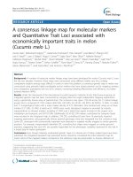
Fig. 1. The construction of NILs through repeated backcrossing. Crossing two genetically
distinct parental lines results in a heterozygous offspring. By backcrossing the heterozy-
gote to the recipient parent, the proportion of donor parental genome is reduced with
50%. In recurrent backcrosses, heterozygosity is further reduced to a small introgression
followed by selfing or sibling mating to obtain a near isogenic line (NIL).
6 R. Kooke et al.
recurrent parent to create lines heterozygous for the introgressed

segment. Crossovers between the homologous chromosomes in
these lines result in recombinants with smaller introgression sizes
which can be phenotyped again to establish the presence or absence
of the QTL in the reduced region. In an iterative process of back-
crossing, recombinant selection, and phenotyping, the QTL is
ultimately reduced to a single or a few genes which can then be
tested using functional genomics approaches.
2.4. Heterogeneous
Inbred Families
A special case of inbred lines are HIFs (3). After crossing two
distinct parents, HIFs are inbred for five or six generations to create
almost complete homozygous genotypes except for a few small
regions (<5% of the genome size) (Fig. 2). A collection of HIFs
can be used like any other mapping population to identify QTLs.
Upon detection of a QTL, however, a single line containing a
heterozygous region coinciding with the QTL but otherwise
homozygous can be selected using the genotypic information of
the population individuals. Progeny of this line will segregate only
for the heterozygous region, creating homozygous lines with dif-
ferent genotypes at the QTL region in a single generation. These
NILs can then be tested to compare the effect of the segregating
region. A hallmark of HIFs is their genomic composition which,
although homozygous, is a mosaic of the two parental lines. This
offers the advantage that often more than one HIF can be selected
which offers the possibility to evaluate the same locus in different
genetic backgrounds. This allows testing QTLs for epistatic inter-
actions with other genomic regions which otherwise can only be
achieved by crossing pure introgression lines (5).
Fig. 2. The construction of heterogeneous inbred families (HIFs). A QTL detected in a RIL
population can be confirmed by the use of HIFs. A predecessor of a RIL which is still

heterozygous for the region of interest but otherwise homozygous is selfed after which the
heterozygous region segregates in a Mendelian fashion. This enables the comparison of
the trait of interest for that specific region for both parental genotypes in an isogenic
background.
1 Backcross Populations and Near Isogenic Lines 7
3. NIL Mapping
Populations
In addition to confirming QTLs detected in mapping populations
or introducing exotic traits in elite breeding lines, NILs can be used
for mapping purposes themselves. A good indication of the pres-
ence of genetic factors explaining differences in quantitative traits is
a comparison of distinct parental lines. In a sense, parental lines
represent the largest possible NILs, i.e., the genome of one parent
is completely replaced by that of another. To detect which part(s) is
responsible for the observed phenotypic variation, the genome
needs to be broken up into smaller introgressed segments divided
over multiple lines which together provide genome-wide coverage.
Depending on the species involved, the available resources, and the
exact purpose of the developed lines, several strategies are in use
which will be outlined below.
3.1. Bulk Segregant
Analysis
Bulk segregant analysis (BSA) is often used in combination with
phenotypic selection strategies (see above). This is probably the
most basic form of genetic linkage mapping as it does not require a
fully genotyped mapping population. Usually a few rounds of back-
crossing and/or inbreeding are sufficient to create a segregating
population. Trait values in such a genetic diverse population often
show a wide distribution range. For qualitative traits, this will be a
binominal distribution according to which the population can eas-

ily be divided into two discrete classes. For quantitative traits,
however, the distribution will approximate normality due to the
larger number of loci involved. Consequently, classifying popula-
tion individuals on the basis of their phenotypes is much more
difficult and arbitrary, but two methods for bulk segregation of
quantitative distributions prevail. The first method simply splits
the population on the basis of the mean, median, or mode (depend-
ing on the skewness) of the distribution. The second method is
more strict and selects only the upper and lower quartile of the
distribution. Both methods have their pros and cons. Splitting uses
all lines of the population, and therefore includes all possible varia-
tion, but might misclassify individuals which reduces mapping
power. Quartile classification, on the other hand, reduces the num-
ber of misclassified lines, but only uses half the population size and
might only detect major effect loci. In all cases, however, two bulks
are formed containing lines of either one of the two designated
classes. In each bulk, all lines are pooled and the two resulting
samples can then be genotyped genome-wide with molecular mar-
kers. Note that markers need to be codominant to quantify allelic
frequencies; alternatively, each individual of the bulk can be geno-
typed separately. Genomic regions enriched for one of the two
parental genotypes in either bulk then indicate QTLs for the trait
8 R. Kooke et al.
of interest. In principle, all segregating populations can be
subjected to BSA, but each will have their own specific properties
(see Chapter 4).
3.2. Genome-Wide
Coverage NIL
Populations
For mapping purposes, NILs are most commonly used as sets of

lines that together span the complete genome sequence (6). For
many species, NILs are often the only alternative for immortal
mapping populations, e.g., RIL populations often suffer from
inbreeding distortion in outcrossing species (see Note 4). The
advantage of NIL populations is that each line contains only a
small section of the donor parent and can directly be compared to
the recurrent parent without the need for sophisticated statistical
tools. The construction of an NIL population covering the entire
genome is a considerable investment and, depending on the use of
the population, one can choose different designs. The largest and
smallest possible introgressions are achieved when whole chromo-
somes (see below) and single-nucleotide polymorphisms (SNPs:
see Chapter 5) are substituted, respectively. Between these two
extremes, there are numerous more possibilities with different
introgression sizes and with different amounts of overlap between
introgression segments (Fig. 3). That said, there are a number of
design issues that affect the mapping power and resolution of NIL
populations. Although there is a large freedom of choice in popu-
lation structures, practical and economic constraints, such as
genome size, generation time, and maintenance or experimental
costs, might direct the ultimate design. An obvious criterion is the
size of the introgressed region in each of the individual NILs.
Smaller introgressions provide a higher mapping resolution, but
Fig. 3. Genome-wide coverage NIL populations. Different population designs can substantially affect population sizes,
resolution, and power. Shown are three different designs, a reciprocal chromosome substitution library, a library with
adjacent large introgressions, and a library with small overlapping introgressions.
1 Backcross Populations and Near Isogenic Lines 9
larger population sizes, i.e., more lines, are needed to maintain
genome-wide coverage. Especially for species with large genome
sizes, this can considerably increase the number of lines to be

maintained and hence experimentation costs. An alternative design
consists of a population of NILs with overlapping introgressions in
such a way that each genomic region is covered twice (or more).
Such a population offers the experimenter the choice to exclude the
overlapping lines at the cost of decreased power and resolution, but
without losing genome-wide coverage (Fig. 3). Finally, one can
choose to develop a one-way or a reciprocal population, i.e., each
parental line serves both as recipient and donor parent in two
separate collections of lines.
Once a certain design has been selected, NILs need to be
developed in a concerted action. After generating an F
1
, this will
usually take several rounds of backcrossing (depending on the
genome size, crossover frequencies (see Note 5 on heterochiasmy),
and desired introgression sizes) followed by one or two generations
of selfing or sibling mating. Eventually, NILs are selected by geno-
typing genomic regions using molecular markers. The efficiency of
NIL construction can considerably be enhanced by using these
markers in what is called marker-assisted selection (MAS). Different
selection strategies have been defined based on marker selection
applied to carrier and noncarrier chromosomes (7, 8). Two-stage
selection is based on selection for the targeted segment on the
carrier chromosome (foreground selection) and against donor
genomic regions on noncar rier chromosomes (background selec-
tion). Three-stage selection involves one more step that selects for
the amount of recombination between the target locus and its
flanking markers and between the flanking markers and the telo-
meres on the carrier chromosome (8). Although in principle a
desired genotype can be selected from a BC

1
population, this
usually requires large population sizes, which exponentially
increases with the genome size (see Subheading 4). Therefore,
having more backcrosses is generally advantageous over genotyping
more lines. Because the level of heterozygosity is highest in earlier
generations, the number of backcrosses can substantially decrease
genotyping costs. However, with each backcross, the average intro-
gression size decreases, which needs to be considered when design-
ing MAS strategies.
An example of using MAS in a crossing scheme could be to use
two-stage selection in BC
1
and three-stage selection in advanced BC
generations, minimizing both genotyping costs and the levels of
donor parental DNA on noncarrier chromosomes (8). On noncarrier
chromosomes, one can increase the number of markers in advanced
generations and only use markers at the telomeres in early generations
to reduce genotyping costs. Eventually all selected lines need to be
genotyped at a resolution high enough to detect double crossovers
(usually 10–20 cM). Finally, all desired lines which are still
10 R. Kooke et al.
heterozygous for the introgressed region after backcrossing should be
inbred to obtain a homozygous immortal mapping population.
3.3. Chromosome
Substitution Strains
A special case of NILs are chromosome substitution strains (CSS):
these carry the largest possible introgression of a single stretch of
DNA into a recipient background. In such a strain, one of the
chromosome pairs of the recipient parent has been substituted

with that of another (donor) parent. Reasons for CSS construction
may be multiple: First, a complete set of CSSs provides a crude
mapping population for QTLs, assigning QTLs to whole chromo-
somes. Second, a CSS removes a lot of background noise from the
population that greatly facilitates identification and fine mapping of
QTLs ((9) and see above). Finally, a CSS provides an excellent
starting point for the generation of smaller NILs. A CSS can be
backcrossed to the recipient parent, introducing heterozygosity on
only one chromosome pair. By subsequent backcrosses, the intro-
gressed segment can be shortened until fixed by inbreeding.
The general approach in constructing CSSs is very similar to
that described for NILs above. An alternative approach that works
well for species with small genomes and large numbers of offspring
is selecting lines carrying a nonrecombinant chromosome 1,
screening the selected lines for a nonrecombinant chromosome 2,
and so on for all chromosomes. This results in the elimination of
approximately 50% of the individuals at every genotyping round,
leaving a BC
1
population from which all CSS can be derived in the
next generation (10).
4. Calculations
Although different criteria may apply for the diverse construction
designs and purposes of NILs and backcross populations, a number
of general rules are instrumental for the development of these
resources. Because most designs follow basic Mendelian genetics,
a standard set of statistical analyses can be applied to calculate
segregation ratios, population sizes, genetic distances, etc.
4.1. Proportions
of Parental Genomes

in Backcrosses
The proportion of each parental genome depends on the number of
backcrosses. The average proportion of the recurrent parental
genome increases with every generation and is given by the for-
mula: ð2
ðbþ1Þ
À 1Þ=2
ðbþ1Þ
or 1 À
1
2
ðbþ1Þ
where b is the number of
backcrosses assuming an infinite population size. The proportion
of the donor genome then simply follows as
1
2
ðbþ1Þ
. Note that these
proportions are independent of genome size and that the fraction
of donor genome halves with every backcross: 50% in the F
1
, 25% in
BC
1
, 12.5% in BC
2
, etc.
1 Backcross Populations and Near Isogenic Lines 11
4.2. Minimal Distance

Between Markers
The genotype of individual lines at specific positions can be identified
by molecular markers (see Chapter 5). The genotype at every other
position, the marker intervals, needs to be estimated from its sur-
rounding markers. To reliably estimate the genotype between two
adjacent markers, their required maximal distance can be calculated.
Incorrect estimates can result from double crossovers between adja-
cent markers which consequently will not be observed. The occur-
rence of double crossovers is therefore dependent on the
recombination frequency between markers, which can be calculated
using Haldane’s mapping function: r ¼
1
2
ð1 À e
ðÀ2d=100Þ
Þ where d is
the distance between markers in cM. From this formula, it can easily
be deduced that the probability of a single crossover event in a 20 cM
region is 17% and a double crossover less than 3%. For a distance of
10 cM, the latter will be even less than 1%. For most purposes, a
genetic distance of 10–20 cM between markers is therefore sufficient
to reliably determine genome-wide genotypes. Note that the rela-
tionship between genetic and physical distances is not constant over
the genome and can vary significantly between species.
4.3. Linkage Drag The number of backcrosses needed to break undesired linkage
between two loci with a given probability again depends on the
genetic distance. The relationship is given by the formula:
N ¼ Log
ð1ÀrÞ
ð1 À PÞ, where N is the number of backcrosses, r is

the recombination frequency, and P is the probability of separation.
To have 95% certainty that a crossover has occurred in a 20 cM
interval would then take 17 ge nerations of backcrossing. E quivalently,
the probability of a crossover to occur between two loci at a given
distance and number of backcrosses would read as P ¼ 1 Àð1 À rÞ
N
.
The chance of a single crossover after four backcrosses over a distance
of 50 cM can then be calculated as 78%. Over a distance of 1 cM, this
would be 4% (11). The examples given here of course represent
random selections of single individuals. In practice, however, multi-
ple individuals are often selected which increases the probability of
crossover occurrence and therefore decreases the number of back-
crosses needed. This is shown by the formula P ¼ 1 Àð1 À p
1
Þ
n
where p
1
is the probability for a single individual and n the number
of selected individuals. The chance that at least one out of ten
individuals carries a crossover in a 1 cM interval after four genera-
tions of backcrossing would then be 34% (compare to 4% for a single
individual).
4.4. Chromosome
Substitution Strains
The generation of CSSs requires the transmission of whole chro-
mosomes, and hence, depends upon the absence of crossovers. The
chance of a certain chromosome not recombining is given by the
function e

ðÀd=100Þ
where d is the length of the chromosome in cM,
while assuming no crossover interference (9). The chance of finding
a specific nonrecombinant donor chromosome in a BC
1
then equals
1
2
e
ðÀd=100Þ
. When one wants to recover an individual carrying a
12 R. Kooke et al.
nonrecombinant donor chromosome with a certainty of q, the
required number of individuals can be calculated by solving
q ¼ 1 Àð1 À
1
2
e
Àd=100
Þ
n
for n.
For CSSs, all other chromosomes need to be of the recurrent
parent genotype. The probability is described by
1
2
ð1 À rÞ
ðcÀ1Þ
where c is the number of chromosomes of the species and r is the
recombination frequency according to Haldane’s mapping func-

tion that assumes no interference between crossover events
(r ¼
1
2
ð1 À e
ðÀ2d=100Þ
Þ where d is the genetic distance in cM) (12).
This probability can estimate the number of individuals that need
to be genotyped in BC
1
to immediately obtain a pure CSS.
The probability of obtaining a CSS is Pða non - recombinant
target chromosomeÞÂP ðall other chromosomes recurrentÞ¼
1
2
e
ðÀd=100Þ
Â
1
2
ð1 À rÞ
ðcÀ1Þ
. From this formula, it can be easily
deduced that the number of individuals to be screened increases
rapidly with the chromosome number of the species. For a species
with only five chromosomes, fewer than 5000 BC
1
individuals need
to be screened to obtain all possible CSSs. For a species with ten
chromosomes, this would require millions of BC

1
individuals, and
multiple generations of backcrossing and selection are therefore
needed.
4.5. Fixing Heterozy gous
Segments
After backcrossing, all introgressed regions are heterozygous, and
therefore selected lines require inbreeding to obtain immortal
homozygous lines. The probability that a progeny carries a homo-
zygous introgression after selfing is given by
P ¼ð1 À rÞ
2
=4 where r¼
1
2
ð1 À e
ðÀ2d=100Þ
Þ
when assuming no interference. The required population size to
obtain the desired genotype with a probability of success q can then
be calculated as: n ¼ lnð1 À qÞ= lnð1 À pÞ (13). For an introgressed
segment of 20 cM, this means that more than 36 individuals (n)
need to be screened to obtain 99.9% confidence (q) of selecting the
desired homozygous line.
5. Notes
1. Congenic strains in animals.
In animals, isogenic lines are often termed congenic strains.
Especially in vertebrates, congenic strains are far more difficult
to produce than, e.g., NILs in plants for a number of reasons.
Vertebrates generally have a much longer generation time with

lower numbers of offspring, suffer from inbreeding depression,
and breeding is more costly. These drawbacks make it almost
impossible to genotype a huge number of individuals and select
1 Backcross Populations and Near Isogenic Lines 13