regional business cycle and real estate cycle analysis and the role of federal governments in regional stability
Bạn đang xem bản rút gọn của tài liệu. Xem và tải ngay bản đầy đủ của tài liệu tại đây (1.05 MB, 120 trang )
Regional Business Cycle and Real Estate Cycle Analysis and
The Role of Federal Governments in Regional Stability
by
Kyoko Mona
A dissertation submitted to the Graduate Faculty in Economics
in partial fulllment of the requirements for the degree of
Doctor of Philosophy, The City University of New York
2008
3325385
3325385
2008
Copyright 2008 by
Mona, Kyoko
All rights reserved
c
2008
Kyoko Mona
All Rights Reserved
This manuscript has been read and accepted for the Graduate Faculty in Economics in
satisfaction of the dissertation requirement for the degree of Doctor of Philosophy.
Professor Christos Giannikos
Date Chair of Examining Committee
Professor Thom Thurston
Date Executive Ofcer
Professor Michael Grossman
Professor Barry Ma
Professor Jeffrey Weiss
Supervisory Commettee
THE CITY UNIVERSITY OF NEW YORK
Abstract
Regional Business Cycle and Real Estate Cycle Analysis and
The Role of Federal Governments in Regional Stability
by
Kyoko Mona
Advisor: Dr. Christos Giannikos
A question how should federal government policy be optimally conducted when
the economy is composed of multitude of states with their own industrial structure is
not a trivial one. Each economy in a multi-state region is characterized by its own
dynamics that, in principle, may be quite different from that of the union in aggregate.
While being quite relevant for the conduct of federal government policy, i.e., monetary
authority, in the United States, the question of optimal monetary policy in a multi-
state economy was disregarded by the modern monetary literature. The objective of
this study is three folds. First, we show that United States is composed in different
economic or multi-state regions. Second, theoretically we show that a uniform policy
by the federal government may not work optimally for each state in multi-state region.
Third, we show that the U.S. is a multi-state region not only in terms for economic
cycles but also in terms of real estate cycles.
This dissertation consists of three essays. Depending on the state level busi-
ness cycles similarity and differences, the rst essay, “The U.S. Regional Business
Cycles Analysis”, divides U.S. into four cyclical regions. The essay shows that some
of the U.S. states have similar business cycles as the nation, while some states have
the opposite cycle patters. Most U.S. states fall somewhere in between. Econom-
ically diminant states have the similar business cycle patterns as the nation. States
with specialized industries often lead the national business cycle patterns. We also
observe that states around the economically dominant states follow or get inuenced
by the economically dominant states's business cycles. Thus, economically not dom-
inant states' geographic proximity from the economically dominant states play quite a
signicant role in the formation of the business cycle patterns of the formar group of
states. The business cycle patterns of the major oil supply states are distinctly different
from the national business cycle patterns.
The second essay of this dissertation, “Optimal Monetary Policy in a Multi-State
Economy”, is a theoretical piece. The results of this essay suggest that when the goal
of the monetary authority is to minimize the variance of some aggregate measure such
as real GDP without explicitly taking the output variance in each region or correla-
tion structure between states into account, it may achieve its goal but may increases
the output variation in regional economies. On the contrary, when the output variance
in each region or correlation structure between states is explicitly included in the ob-
jective function, the model not only successfully reduces the output variances in the
states but also reduces the national output variation.
The third essay, “Are U.S. States Economic and Real Estate Cycles Related”,
found that there are no distinct and persistent patterns between real estate cycles and
state level economic uctuations. We observe that real estate downturns are more
persistent and severe than economic recessions. Comparison of the national and state
level business and real estate cycle patterns suggest that only two out of four recent
NBER dated national recessions were accompanied by predominance of real estate
downturns in most of the U.S. states. Our results also suggest that nearly forty U.S.
states as well as the U.S. on aggregate exhibited distinct downturn of the real estate
cycle between the third quarter of 2006 and the rst quarter of 2007. Finally we found
that the state level economic and real estate growth rate diverges during the period of
recession.
Acknowledgments
I would like to gratefully acknowledge the contributions of those without whom
this dissertation could not have been completed.
First and foremost, I would like to express my gratitude to my principal advisor
Professor Christos Giannikos. He has been my mentor, guide and friend for last two
years when I started working with him. His role towards my nishing up dissertation
is very signicant. Without his support and motivation I would have never nish up
my Ph.D.
I would also like to thank Professor Barry Ma and Professor Jeffray Weiss to
be in my dissertation committee. Both Professor also been my mentor throughout
my graduate school and provided me with invaluable direction, advice, help and com-
ments.
I must thank my initial advisor Professor Howard Chernick for introducing me
the topics of Public Finance. Without his teaching, mentoring and guidance I would
never able to nd my dissertation topic.
I would also like to thank Professor Thom Thurston and Professor Michael
Grossman for their continuous support. Their kindness, care and concern are un-
matched. Both Professors believed in me and gave me strength throughout my time in
graduate school. Without their support and care I would never be able to survive in the
graduate program.
I am also grateful to Professor Harsey Friedman, Professor Merih Uctum, Pro-
fessor Kishor Tandon and Dean Zadra for giving me the exceptional opportunity to
support myself throughout my graduate study.
I would like to acknowledge all those who made my graduate school experience
enjoyable, and memorable. Dianne (APO of the GC Economic department); Terissa,
Maria, and Irina (Cafetaria Staffs); Allison, and Sylvia (Secretaries at Baruch College);
and Mr. Dauglas Ewing and other staff members of the International Student Service.
I must also thank Ms. Judy Waldman to go over my thesis at the last moment.
I would like to thank all my friends at the Graduate Center, Eric, Esin, Francois,
Fredy, Fued, Julio, Mete, Nadia, Ozlem, Patrik, Raed, Skye, Xuli, and Yoko to take a
ride together. I would also like to thank my friends out side the Graduate Center for
their support and understanding, Fahm, Emu, Fate, Nubras, Nusrat, Topu, and Shar. I
must thank Ben and Nicklina for going over my dissertation and proof reading it.
I would also like to thank my family members, all my cousins, aunts, uncles
and in laws to stand by me. Specially I must mention Bora and Kakoly auntie, who
always shared their home with me. I must thank Moni chacha who took care of my
father's unnished business so that I did not have to think about those. Also, I thank
Yamamoto family in behalf of my family to stand by us throughout the difcult time
of our lives. I am lucky to be a part of this family. I specially thank three of my sisters
Ahrita, Lisa, and Shanta apu to be the closest person in my life. All my love to David,
Lilit, Nafee, and Ontor who always reminded me what a beautiful place the world is.
Finally, I want to dedicate this dissertation to ve very special people in my
life, who played a signicant role reshaping it. First, my home tutor Moqbul Hassan,
without him I would not learn to read and to write. Moqbul Sir gave me eyes with
which I learned to see. Second, my undergraduate management professor, Dean Don-
ald Mosley who gave me light. Professor Mosley helped discover my true self. Third,
I thank my mother, without her nancial and mental support nothing would happen.
She is the air in my life. Forth, I would like to thank my father and grand father who
have already build a path for me. Life was comparatively easier for me because I just
had to follow their path. Finally, I would like to thank my dearest friend and sole mate
Aram, who was the greatest company in this journey.
Contents
1 Introduction . . . . . . . . . . . . . . . . . . . . . . . . . . . . . . . . . . . . . . . . . . . . . . . . . . . . . . . . . . . . . 1
2 The U.S. Regional Business Cycles Analysis . . . . . . . . . . . . . . . . . . . . . . . . . 6
2.1 Introduction . . . . . . . . . . . . . . . . . . . . . . . . . . . . . . . . . . . . . . . . . . . . . . . . . . . . . . . . . . . . . 6
2.2 Literature Review . . . . . . . . . . . . . . . . . . . . . . . . . . . . . . . . . . . . . . . . . . . . . . . . . . . . . . . 9
2.3 Data . . . . . . . . . . . . . . . . . . . . . . . . . . . . . . . . . . . . . . . . . . . . . . . . . . . . . . . . . . . . . . . . . . 12
2.4 Model and Estimation Method . . . . . . . . . . . . . . . . . . . . . . . . . . . . . . . . . . . . . . . . . 13
2.5 Results . . . . . . . . . . . . . . . . . . . . . . . . . . . . . . . . . . . . . . . . . . . . . . . . . . . . . . . . . . . . . . . 18
2.6 Conclusion . . . . . . . . . . . . . . . . . . . . . . . . . . . . . . . . . . . . . . . . . . . . . . . . . . . . . . . . . . . . 29
2.A Appendix . . . . . . . . . . . . . . . . . . . . . . . . . . . . . . . . . . . . . . . . . . . . . . . . . . . . . . . . . . . . . 31
3 Optimal Monetary Policy in a Multi-State Economy . . . . . . . . . . . . . . 45
3.1 Introduction . . . . . . . . . . . . . . . . . . . . . . . . . . . . . . . . . . . . . . . . . . . . . . . . . . . . . . . . . . . 45
3.2 Literature Review . . . . . . . . . . . . . . . . . . . . . . . . . . . . . . . . . . . . . . . . . . . . . . . . . . . . . 48
3.3 The Model . . . . . . . . . . . . . . . . . . . . . . . . . . . . . . . . . . . . . . . . . . . . . . . . . . . . . . . . . . . . 50
3.3.1 National Variation Analysis . . . . . . . . . . . . . . . . . . . . . . . . . . . . . . . . . . . . . 52
3.3.2 Regional Variation Analysis . . . . . . . . . . . . . . . . . . . . . . . . . . . . . . . . . . . . . 55
3.4 Results . . . . . . . . . . . . . . . . . . . . . . . . . . . . . . . . . . . . . . . . . . . . . . . . . . . . . . . . . . . . . . . 57
3.4.1 Comparison of the national output variation . . . . . . . . . . . . . . . . . . . . . . 60
3.4.2 Does
separate
reduce one region's output variance? . . . . . . . . . . . . . . 60
3.4.3 Does
aggregate
increase one region's output variance?. . . . . . . . . . . . . 61
3.5 Conclusion . . . . . . . . . . . . . . . . . . . . . . . . . . . . . . . . . . . . . . . . . . . . . . . . . . . . . . . . . . . . 64
3.A Appendix . . . . . . . . . . . . . . . . . . . . . . . . . . . . . . . . . . . . . . . . . . . . . . . . . . . . . . . . . . . . . 65
4 Are U.S. States Economic and Real Estate Cycles Related? . . . . . . 68
4.1 Introduction . . . . . . . . . . . . . . . . . . . . . . . . . . . . . . . . . . . . . . . . . . . . . . . . . . . . . . . . . . . 68
4.2 Literature Review . . . . . . . . . . . . . . . . . . . . . . . . . . . . . . . . . . . . . . . . . . . . . . . . . . . . . 70
4.3 Data Descriptions . . . . . . . . . . . . . . . . . . . . . . . . . . . . . . . . . . . . . . . . . . . . . . . . . . . . . 72
4.4 Model and Estimation Method . . . . . . . . . . . . . . . . . . . . . . . . . . . . . . . . . . . . . . . . . 73
4.5 Result . . . . . . . . . . . . . . . . . . . . . . . . . . . . . . . . . . . . . . . . . . . . . . . . . . . . . . . . . . . . . . . . 76
4.6 Convergence Analysis . . . . . . . . . . . . . . . . . . . . . . . . . . . . . . . . . . . . . . . . . . . . . . . . . 86
4.7 Conclusion . . . . . . . . . . . . . . . . . . . . . . . . . . . . . . . . . . . . . . . . . . . . . . . . . . . . . . . . . . . . 91
4.A Appendix . . . . . . . . . . . . . . . . . . . . . . . . . . . . . . . . . . . . . . . . . . . . . . . . . . . . . . . . . . . . . 93
Bibliography . . . . . . . . . . . . . . . . . . . . . . . . . . . . . . . . . . . . . . . . . . . . . . . . . . . . . . . . . . . . . . 105
List of Figures
Figure 2.1 50 U.S. States GSP Growth rate, 1987 - 2002 . . . . . . . . . . . . . . . . . . . . . . . 8
Figure 2.2 The U.S. Business Cycle Turning Points . . . . . . . . . . . . . . . . . . . . . . . . . . 19
Figure 2.3 California . . . . . . . . . . . . . . . . . . . . . . . . . . . . . . . . . . . . . . . . . . . . . . . . . . . . . . . 22
Figure 2.4 Colorado. . . . . . . . . . . . . . . . . . . . . . . . . . . . . . . . . . . . . . . . . . . . . . . . . . . . . . . . 24
Figure 2.5 Wyoming . . . . . . . . . . . . . . . . . . . . . . . . . . . . . . . . . . . . . . . . . . . . . . . . . . . . . . . 25
Figure 2.6 Maryland . . . . . . . . . . . . . . . . . . . . . . . . . . . . . . . . . . . . . . . . . . . . . . . . . . . . . . . 26
Figure 2.7 Pennsylvania . . . . . . . . . . . . . . . . . . . . . . . . . . . . . . . . . . . . . . . . . . . . . . . . . . . . 28
Figure 3.1 Correlation Between State Outputs . . . . . . . . . . . . . . . . . . . . . . . . . . . . . . . 59
Figure 3.2 Output Variance in State One With No Policy . . . . . . . . . . . . . . . . . . . . . 63
Figure 4.1 The U.S. Business and Real Estate Cycles . . . . . . . . . . . . . . . . . . . . . . . . 78
Figure 4.2 California's Real Estate Cycle Analysis. . . . . . . . . . . . . . . . . . . . . . . . . . . 80
Figure 4.3 Maryland's Real Estate Cycle Analysis . . . . . . . . . . . . . . . . . . . . . . . . . . . 82
Figure 4.4 Maine's Real Estate Cycle Analysis . . . . . . . . . . . . . . . . . . . . . . . . . . . . . . 83
Figure 4.5 Mississippi's Real Estate Cycle Analysis . . . . . . . . . . . . . . . . . . . . . . . . . 85
Figure 4.6 Convergence Analysis . . . . . . . . . . . . . . . . . . . . . . . . . . . . . . . . . . . . . . . . . . . 87
Figure 4.7 Real Esate Fluctuations and Severity Analysis . . . . . . . . . . . . . . . . . . . . 88
Figure 4.8 Economic Fluctuation and Severity Analysis . . . . . . . . . . . . . . . . . . . . . . 90
1
Chapter 1
Introduction
When the National Bureau of Economic Research (NBER) announces reces-
sion for the country what does it really mean? Does this recession picture true for
every regions of the country? In another word, when Macroeconomic data show
a picture of economic expansion for a country, do every regions of that country
share the same expansion or do certain regions suffer recessions that the govern-
ment ignores? For example, from 1990 to 1993, during the national recession, state
of Michigan experienced economic expansion; where as, from 1993 to 2000, when
the U.S. economy started picking up, the Michigan's economy went into recession.
The similar outcome we experienced in Pennsylvania during 1995 – 2000. The U.S.
economy was in expansion while, the Pennsylvania's economy was facing a reces-
sion.
What causes regional business cycle? Is it specic to a type of industry in a
state or general government policy implication? How different these cycles are in
state to state? Let us assume that during national recession, to stabilize the over all
economy, the federal government chooses a set of economic policy. Does this unique
national policy adversely affect the growth of states like Michigan and Pennsylvania
because those states have state specic business cycles which always do not coincide
with the national business cycles? Do government policies for a national recession
2
worsen the economic condition of the state like Michigan and Pennsylvania in the
subsequent period? Then, to what extent should the highest level of government
get involve with the regional economy? Are there any relationships between state
level business cycles and federal government policy implications, which may affect
national growth in the long run?
These are very obvious questions for a Multi-state region like the United States.
In recent years a considerable research had been conducted specially on the European
regions in the application of if the European Union is an optimal currency area. How-
ever, there is very few, if any, research on the U.S. optimum currency area in recent
years which deals with regional economic uctuations. We believe that revisiting
the topic of if the U.S. is an optimal currency area and nding the similarities and
the differences in regional business cycle patterns are important areas to explore for
three notable reasons: 1) it will give a vivid idea about regional business cycles to
the future economists and researchers; 2) we can re-explore the question if an unique
monetary policy decision works optimally in each regions of the United States; 3)
it will assists future government policy makers to come up with a better monetary
policy goal function to reduce regional economic uctuations.
This dissertation is consists of three essays. The rst essay is presented in
chapter two which, focuses on the regional business cycles. We dene the U.S. states
as a region. Using Hamilton's Markov Switching estimation technique on the U.S.
fty states coincident indexes, we calculate the turning points of the state level busi-
3
ness cycles. We observe that the state level business cycle varies not only from each
other but it also varies from the national business cycle. Depending on the pattern of
the state level business cycle we divide the U.S. into four major cyclical regions. In
one extreme we found that economically dominant states, e.g., New York and Cali-
fornia, have similar business cycle patterns as the U.S. On the other extreme, some
states have opposite business cycle patterns compared to the national business cycle
patterns. States with specialized industries often lead the national business cycle pat-
terns. Further, we observe that states around the dominant economic states follow
or get inuenced by the dominant economic state's business cycles. Thus, econom-
ically not dominant states' geographic proximity from the economically dominant
states plays quite a signicant role in the formation of the business cycle patterns of
the former group of states. The business cycle patterns of the major oil supply states
are distinctly different from the national business cycle patterns.
The second essay of this dissertation is a theoretical piece, which is presented in
the chapter three. In the rst essay we observe that each state in the United State has
state specic business cycles, which may or may not coincide with the national level
business cycles. Thus we pose a question that what should be the optimum monetary
goal function for an economy which is composed of a multitude of states with own
industrial structure. This essay sets forward a formal analysis of optimal monetary
policy in a multi-state economy by using a simple IS-LM model. For simplicity
of analysis we assume a two-states economy. Therefore, our model modies the
4
Hicksian IS-LM framework by using two IS curves – one for each regional economy
– and one LM curve for the nation. We suggest a new monetary policy goal function
that is more suitable for the case of a multi-state economy. This modied framework
not only takes into account the regional output variance but also allows for more in-
depth analysis of the correlation structure between states. The results of this essay
suggest that when the goal of the monetary authority is to minimize the variance
of some aggregate measure such as real GDP without explicitly talking the output
variance in each region or the correlation structure between states into account, it may
achieve its goal but may increases the output variation in regional economies. Unlike
this, when the output variance in each region or the correlation structure between
states is explicitly included in the objective function the model not only successfully
reduces the output variances in individual states but also reduces the national output
variation. In fact the later model outperforms the former one as long as the correlation
factor between state outputs is greater than negative one.
In chapter four we present the third essay. In the third essay we try to analyze if
certain industrial cycle has specic contribution towards states level economic cycles
and the U.S. national business cycles. As a representation of a random industry, we
analyze real-estate industry of the United States for two main reasons: one, real es-
tate is one of the dominant industry sectors of the United State; and two, a recent U.S.
housing market uctuation triggered a question about what is the impact of uctua-
tions in the real estate market on the U.S. economy. This essay uses Markov Switch-
5
ing estimation technique on U.S. state level coincident index and housing price index
to indicate state as well as national business and real estate cycles. The analyses in
this essay suggest that there are no distinct and persistent patterns between real estate
cycles and state level economic uctuations. We observe that real estate downturns
are more persistent than economic recessions. Comparison of the national and state
level business and real estate cycle patterns suggest that only two out of four recent
NBER dated national recessions were accompanied by predominance of real estate
downturns in most of the U.S. states. Our results also suggest that nearly forty ve
U.S. states as well as the U.S. on aggregate exhibited distinct downturn of the real
estate cycle between the third quarter of 2006 and the third quarter of 2007. Severity
of state level real estate uctuations, measured in this paper as a difference between
growth rates in expanding and declining phases, varied remarkably across states. We,
however, observe relatively greater dispersion of the growth rates of the state hous-
ing index when the states economies are in recessionary phase of the business cycle.
This suggests that the housing market across states converges during periods of ex-
pansions. The same outcome holds for the state coincident index.
6
Chapter 2
The U.S. Regional Business Cycles Analysis
2.1 Introduction
The National Bureau of Economic Research (NBER) calculates and produces
business cycle turning points for the U.S. economy at the aggregate level
1
. Accord-
ing to the business cycle studies, a country's economic condition can be divided into
two phases of a business cycle – expansion and recession. Many economic stud-
ies and policy makers take this aggregate business cycle phases
2
by NBER as given
while making policy decisions for the nation. Some evidences, however, show that
when central policy makers, namely the Central Bank, make uniform decisions for
the nation based on the aggregate business cycle conditions, these policies may or
may not work uniformly throughout the U.S. regions. For example, during 1985
the U.S. economy was in expansionary phase of the business cycle whereas some
states, i.e., Idaho, Iowa, Louisiana, Oklahoma and some other states were in a reces-
sionary phase. During that time, from 1985:I quarter to 1985:IV quarter the Central
Bank chose contractionary monetary policy and the fed-funds rate went up gradually
1
/>2
Lag indicator
7
throughout the expansionary period
3
. High fed-funds rate made recession worse in
states and regions which were facing recessionary phase of the business cycle. Some
recent business cycle studies start questioning about the aggregate measures of the
business cycles and start looking into the state level and the regional level economic
conditions, i.e., Crone [14]; Kouparitsas and Nakajima [22]; Owyang, and Piger [27].
In this essay we used Markov Switching estimation technique on the U.S. fty
state coincident index to calculate the business cycle turning points for all fty states.
In this way we will have state level business cycles, which can be compared with the
national business cycle. This is an important study, especially for a nation consisting
of multiple regions, e.g., the U.S., Canada, EU, China, and Russia, for two reasons.
First, without having a clear idea about the regional business cycles, a uniform de-
cision by the national government based on GDP data may adversely affect some
regions, which may have different business cycles than that of the nation. Second, a
clear understanding about the state/ regional level business cycles will help various
governments to take appropriate measures to reduce the impact of recession.To jus-
tify our point, that the different regions in a multi-state economy may face different
phases of the business cycles we plot Figure: 2.1. In other words, some regions may
experience positive growth, while other regions may experience negative growth. In
Figure: 2.1, we plot growth rate of GDP and Gross State Product (GSP) for U.S. fty
states from the 1987 to the 2002 time period. The Figure: 2.1, shows that the growth
3
/>8
Figure 2.1: 50 U.S. States GSP Growth rate, 1987 - 2002
-0.06
-0.04
-0.02
0
0.02
0.04
0.06
0.08
1986 1988 1990 1992 1994 1996 1998 2000 2002
Year
Growth Rate
Alabama Alaska Arizona Arkansas California Colorado Connecticut Delawar
DC Florida Georgia Hawaii Idaho Illinois Indiana Iowa
Kansas Kentucky Louisiana Maine Maryland Massachusetts Michigan Minnesota
Mississippi Missouri Montana Nebraska Nevada New Hampshire New Jersey New Mexico
New York N Carolina N Dekota Ohio Oklahoma Oregon Pennsylvania Rhode Island
S Carolina S Dakota Tennessee Texas Utah Vermont Verginia Washington
W Verginia Wiacinsin Wayoming USA
9
rate throughout the states varies and the state level growth rates are different from the
national growth rate. For example, during the 1987 and the 1988, the U.S. was fac-
ing positive growth rate while the state of Alaska was facing negative growth rate.
Later, from the 1988 to the 1989 the U.S. economy started facing negative growth
rate, while Alaska started experiencing the opposite.
In the following sections, rst we go over some related literatures; second, we
explain the data used in this essay; third, we present the model and methods; fourth,
we provide results; and we conclude in section ve.
2.2 Literature Review
Exuberant researches by the Federal Reserve Bank and the Bureau of Economic
Analysis (BEA) indicate that the U.S. can be divided into six, eight, or twelve eco-
nomic regions depending on their geographical locations, population density, socio-
economic conditions, and`industry structures and the like. Until early 1990's, these
regional groupings were used heavily by the monetary and scal authorities for de-
cision making purposes and by the researchers for economic analysis. Applying
cluster analysis on Stock and Watson's coincident indexes [31], recently Crone [12]
observed monthly changes in economic activities in all fty different states. His re-
search shows that states economic conditions vary a lot compared to each other and
from the aggregate economy. While many researchers still use the eight or twelve di-
10
visions of economic - geographical regions, most researchers these days treat states
as a complete economic region in the United States.
Starting from mid 1990's many researchers used the Vector Autoregression
(VAR) models to analyze the different effect of monetary and scal policy on the re-
gional economies. Carlino and DeFina [5], [6]; Clark [10]; Owyang and Wall [28];
and Crone [14] found that due to various industry structures, banking systems, shock
absorbing mechanisms, different regions act differently when the Federal Reserve
Bank changes the interest rates. Most of these studies took the BEA classication of
regions as given and analyzed regional business cycles phenomena based on similar-
ities at a point in time.
From the other perspective a study by Wall and Zoega [34] tried to show that
aggregate gures may not reect all the regions in the United State at the same time.
For example during the 1981-82 recession the U.S. unemployment rate rose by about
3.3 percentage points from the third quarter of 1981 to the fourth quarter of 1982.
During the same period, twenty nine states had smaller increases, fourteen states had
almost no change, one state decreased, and six states had a rise more than 4.8 per-
centage points in their unemployment rate. Similarly, they showed that during the
1990 – 1991 recession aggregate unemployment rate rose by 2.3 percentage points
from the second quarter of 1990 to the third quarter of 1992. Regional data, however,
show that only California, New York, North Carolina, and Washington faced similar
rise in the unemployment, whereas thirty six states experienced very mild increase in
11
unemployment, and for the rest of the states unemployment rate decreased. Similarly,
during the 2001 recession, which began in the fourth quarter of 2000 and continued
until the end of 2002, aggregate unemployment rose 1.6 percentage points, although
thirty ve states experienced smaller increase than the aggregate gure and six ex-
perienced a decline in the unemployment rate. Thus, Wall and Zoega [34] conclude
that each state may vary differently from the nation.
Boldin [3] compares ve different business cycles turning point dating methods
on the U.S. economy and concludes that the Stock and Watson's [31], [32] experi-
mental business cycles indicators based on Kalman lter algorithm and Hamilton's
[20] Markov Switching estimation technique outperform all other business cycles
dating techniques. Following Boldin [3], using Markov Switching estimation tech-
nique on Crone's [13] state indexes, Owyang, Piger, and Wall [27] in their recent
paper
4
showed that each state experiences its own business cycles, while state level
business cycles not necessarily coincide with the national business cycles. Further,
they show that the recession growth rates are related to the industry mix, whereas the
expansion growth rates are related to education and age composition.
4
This study is very close to the Owyang, Piger and Wall (2005) paper. We started writing this paper
in 2004 without knowing the work of Owyang, et al.'s paper. In 2005, we found out that Owyang,
et al. had already gotten their paper published. Nevertheless, our basic Markov Switching model is
slightly different from the model suggested by Owyang, et al. Also we extended the time period until
2007:IVQ. Finally, our ndings and the way we conclude this study is different from the study done
by Owyang, et al.
12
A recent study by Crone [14] also estimates the U.S. state level business cycles
using the diffusion indexes. His study concludes that the diffusion indexes are better
data sets to track or to forecast regional business cycle turning points.
2.3 Data
We used the U.S. 50 states coincident indexes provided by the Federal Reserve
Bank of Philadelphia dating from 1979:IQ – 2007:IVQ. This data set is developed
by Crone [12] estimating four latent dynamic factors of each state. The four vari-
ables are: the total number of jobs in nonagricultural establishments, average weekly
hours in manufacturing, the unemployment rate, and the real wage and salary dis-
bursements. This is one of the most comprehensive monthly data set available for the
state level economic analysis. The reason for using the state level coincident indexes
for the study is that there is no monthly Gross State Product (GSP) data available for
the U.S. states. The available GSP data are in the annual basis, but the state level
recession can begin and end within a year.
In addition to the state level business cycles, we also re-estimate the turning
points of the national business cycles for two notable reasons. First, we want com-
pare our estimated national business cycles turning points using Markov Switching
estimation technique to the national business cycles turning points dates given by
the National Bureau of Economic Research (NBER). This comparison will prove the
authenticity of the measuring technique. Second, we want to compare the national