Cs224W 2018 46
Bạn đang xem bản rút gọn của tài liệu. Xem và tải ngay bản đầy đủ của tài liệu tại đây (6.28 MB, 9 trang )
Graph Analysis of Major League Soccer Networks:
CS224W Final Project
Evan Huang! and Sandeep Chinchali*
'Stanford University
Stanford University
December 9, 2018
1
Introduction
(GCNs)
Given the natural existence of networks in teambased sports, we hope to use network analysis and
predictive modeling to better analyze soccer. Currently, research in soccer analytics has focused on
individual player statistics, and predictive modeling
has been limited to simple logistic regression, decision trees, and LSTMs
[3]. We believe that leverag-
ing network structure will create better results given
the importance of teamwork within the sport. In particular, a better predictive model can benefit both the
sports betting industry (last year, the total betting on
sport was $4.9 billion in Nevada alone [1]) and the
soccer team’s management.
As such, we hope to learn how the network structure of a soccer team can be exactly leveraged to
predict end of game results. Given the differences
in teams, players, and strategies, creating a general
approach based on given network information is not
straightforward. Therefore, we hope to come up
with a particular approach and model to augment
current predictive techniques.
2
Related Work
One of our main novel contributions in this project
would be assessing whether graph-based learning algorithms like Graph Convolutional Networks
[2] perform
better than
other
traditional
learning algorithms in the context of prediction and
analysis of sports games.
There has been some related work in sports analytics conferences like the MIT Sloan Sports Analytics conference; for example, one paper [3] describes data-driven ghosting in soccer games which
enables coaches and managers to “scalably quantify,
analyze and compare fine grained defensive behavior’. Their learning task was different than our proposed one here because they were more interested in
analyzing and modeling player movements and defense styles, not predicting game statistics. Other related work includes an MIT Master’s Thesis [4] and
a journal paper [5] which also use similar data from
soccer games to infer passing patterns and styles
[4], assess players’ passing effectiveness, and predict shots [5].
However,
to the best of our knowl-
edge, none of these papers represent the data as a
network graph and utilize the graph structure in their
inferences, which is where our current work is situ-
ated.
3.
Overview and Contributions
Principal Contributions: To our knowledge, predicting soccer game outcome from play-by-play
data using a passing rate graph and feature embeddings such as node2vec and Graph Convolutional
Networks
(GCNs)
has never been done before.
A
principal contribution of our project is to use hardto-obtain, high quality play-by-play data to compare
the predictive power of simple features with those
based on random walk simulations and deep learning.
Paper organization: The rest of our paper is organized as follows. In particular, our overall soccer
graph analysis pipeline is illustrated in Figure 4:
We
collected
the
annotated
data
from
OPTA,
a sports analytics company, which ensured data
fidelity and annotated player actions (passing,
aerial shots) using uniform video annotation techniques. Overall, the dataset consists of 2,280 games
from players across 60 diverse teams, leading to
3,893,304 player actions (rows). Since only one
player is considered in each timestep, we can identify player A passed to player B by considering the
action and players in successive timestamps.
1. Graph Creation:
We describe our data sanitization and graph
creation process in Section 4, with an example
graph in Figure | and basic dataset statisics in
Figure 2.
2. Node Feature Embeddings:
In Section 5,
we introduce a variety of techniques to learn
key features of nodes that are used to predict game
outcome,
summarized
in the over-
all results table of Figure 7. We also investigate whether these features are discriminative
enough to cluster games using t-SNE by either
game outcome (Figure 5) or team identity (Figure 6).
3. Graph Convolutional Neural Network:
Fi-
nally, in Section 6, we use a custom random-
walk procedure to learn node embeddings
using Graph Convolutional Neural Networks
(GCNs) that are the best-performing on game
outcome prediction.
4
Dataset and Graph Structure
Our dataset consists of 6 seasons of “play-by-play”
soccer games from major professional leagues such
as Li Liga (Spain), English Premier League (EPL),
and Major League Soccer (MLS). For a given game
between two teams, “play-by-play” data identifies
each player, their x and y coordinates in the field,
a timestamp of hour, minute,
and second,
and the
major action taken by that player, such as a pass,
interception, aerial shot, goal etc. in a standardized
vocabulary.
4.1
EPL Dataset
We test our models on the EPL dataset before aggregating other datasets. The EPL dataset consists of
a single season in 2012, consisting of 380 matches
between 20 teams, such as Liverpool, Manchester
United, Southampton, etc. The dataset consists of
648,883 unique plays made by 524 unique players,
who are annotated to have 5 positions of Strikers,
Defenders,
tutes.
Midfielders,
Goalkeepers,
and
Substi-
Each play is annotated using a standardized
vocabulary of 46 actions, including “Goals” and ‘In-
terceptions”.
4.2
Graph Structure
The team structure within a given match is represented as a weighted, directed graph, where nodes
are players and edges are actions (pass, kick, etc.).
Our initial networks also include additional event
nodes to represent non-player states such as the
gaining of the ball, the loss of a possession, and a
shot taken. Respectively these are named “Gain”,
“Loss”, “Shot’’, and “Goal”.
Nodes: 14 to 17 nodes consist of 11 players from
each team plus events and substitute players.
Edges: If player (node) A passed to player B
(node B) some
amount
of times within a game,
a
passing edge is created. Concurrently, shot, gain,
and loss rates are also used to connect player nodes
to event nodes. The weights on the edges can be
formulated as follows:
1. Passes (A, B) = (num. successful passes between A and B) / (time shared between A and
B)
2. Shots(A) = (num.
saved attempts, post hits,
misses, or goals) / (time A on field)
3. Gain(A) = (num. of ball recoveries, corners
awarded, out of bounds rewarded) / (time A on
field)
4. Loss(A) = (num. unsuccessful passes, out of
bounds, dispossessions) / (time A on field)
1.0,
1. Single game networks with 2 teams.
Each
team is connected through respective losses
and gains of possessions, transforming original
“Gain” and “Loss” nodes into “Switch” nodes.
2. Aggregated team network consisting of data
within a whole season. Each team’s individual
networks is aggregated across all games, giving one unique network per team. Rates are
now based on total time rather than time in a
game.
0.8
Ultimately, we decided to use our single game
structure for predictive purposes. That is, we want
to know whether passing rates within a single game
retains enough information to accurately predict that
specific game’s results.
0.6Ƒ
0.4E
0.2F
0.0}
0.2
0.0
0.2
0.4
0.6
0.8
1.0
1.2
Figure 1: Example Graph Structure for a Single
Team in a Single Game. Player nodes are colored
in cyan and edge weights (passing rates) are omitted for visual clarity.
Goal
distro.
by player for scorers
(at least 1 goal)
Number
_
e
©
of players
_
N
©
140
80
4.3
Data Processing
Our code processes the play-by-play data using 2
pointers that track players making actions, and players receiving actions. Time on field is measured
through substitution events, where in the event a
substitution doesn’t occur, the player is assumed
to have played the whole game. These counts of
actions are stored in a dictionary representing an
edge list where keys are tuples of player IDs. The
time metrics are then used to transform these dictionary components into rates. Additional information
tracked include team, home
60
winning team, and match id.
40
20
0
5
10
Number
15
of Goals
20
25
Figure 2: Per-player goal distribution across a season.
Two additional networks were considered to represent a single team in a single game, such as:
vs away status, goals,
As a sanity check, we plotted the distribution of
goals across a season for EPL players that scored
at least once. Figure 2 shows a reasonable distribution between 1 goal (the mode) and a maximum
of 26 per-player season goals. Figure 3 illustrates a
reasonable distribution of aggregate goals per team
across a season, given each team likely scores
1-2
goals in each of its approximately 20 games. The
edge list dictionary is used to create a passing-rate
weighted TNEANet graph in SNAP.
5.2
Number of teams
N
U
b
Goal distro. by team across season
Graph Clustering
ture Vectors
from node2vec per team, we wish to cluster them
_ˆ
to discover latent relationships or whether they aggregate based on outcome (‘win’, ‘loss’, “draw”) or
team identity. Since each team plays 20 games, we
have several realizations of a team’s playing style.
50
60
Number of Season
70
Goals
We used the standard t-SNE method [9] for clus-
80
tering since it can be projected to two dimensions
for easy
Figure 3: Per-team total goal distribution across a
season.
Graph
Analysis
and
Node
Node
Embed-
Feature Embedding
5.1
Feature
dings
Learning:
first embedding,
visualization.
Further,
its probabilistic
assignment of cluster membership is attractive in
the soccer context since teams likely have dynamic
playing styles based on their opponent, current substitutions, and even whether they are the home team.
We implemented t-SNE using python’s sklearn
package and visualized the embeddings in two dimensions for both simple and node2vec features.
Per feature set, we ran t-SNE twice, once on a ma-
trix where rows were matches and columns where a
single team’s features, and again where rows were
Given our goal to predict game results and/or analyze teams effectively, we want to learn node embeddings from our graphs that maximimize predictive and discriminative power.
Our
on Fea-
Given both simple hand-crafted features and those
40
5
Based
which
we
call simple
or
matches and columns concatenated both the home
and away team’s vectors. The latter is more useful to predict outcome since it contrasts the playing
style of both teams.
We rigorously applied t-SNE using best practices
such as sample normalization to account for the dif-
hand-crafted features, sets the average pass rate,
max pass rate, min pass rate (nonzero), shot rate,
gain rate, and loss rate in a vector for each node.
We then can assemble a feature vector for a specific
graph by averaging the features of the node within
the graph.
ferent scales of input variables. Initially, we found a
Our second embedding uses node2vec [7] with
default parameters (128 dimensions, 80 length walk,
10 walks per source, weighted directed graph) to retrieve a feature vector per node. The feature vectors
are then averaged to obtain a feature vector for a
graph.
to substitutions. Also, we sometimes saw two clusters, which were later learned to be for ‘home’ and
Our current node aggregation technique is simple,
but may lose a lot of information. Therefore, we
hope to learn more rich, higher-order interactions
between players, using a more complex model such
home/away team status, we realized t-SNE did
not help in clustering the data, as shown below.
as a GCN
[2,6].
few clusters, though they did not separate based on
our desired goal of predicting game outcome.
Upon further analysis of nodes in each cluster,
we realized that the clusters corresponded to cases
where teams had 14,15,16, or 17 players overall due
‘away’ games but were still not predictive of game
result. Examples of such uninformative clusters are
provided below.
However,
when omitting number of players or
Crucially, rather than simply averaging individual
player feature vectors, we will subsequently learn
more predictive features from them using GCNs.
1. Raw Play-By-Play Data
3. Feature Learning
4. t-SNE Clustering
T-SNE on home and away team embeddings (normalized)
Player
Team
Play
Attempt
B
—
x
Man. U
Pass
Fail
Liverpool
Goal
Success
A
“Sone
30
=>
zoj
10
gfe
oe
t9
acre
°
ee
sec oe € 9
4+
0
2. Graph Extraction
*
-ao |
3
Sets: &,
2+ . e
đẫ,ề$
EPO hh
pe
eo,
.
ee
h$
ress
#
y
oe
a
SB -
cect
og?
â 068
dag 829 ageeđ e
e ° 2%
-20
=
r
=
Sgt, Ya
-10
node2vec
ee
Sree
Ve
›
®
“s
di
ee
home win
home loss
“
cs
ee
s
oF
À
|
er HS
a
L7
q
phon
b.
Ss
2%
ý BERL
CCTMe
1[KAZ
S
4
cá 5s
6 NI
y
A
⁄
IAS
L
aT
& wg
X
CC
ch
Figure 4: Soccer network analysis pipeline starting from (1) play-by-play data, (2) passing rate graph
extraction, (3) feature embedding, (4) clustering, and finally (5) game result prediction. We compared the
predictive utility of simple, domain-specific features with complex ones learned by Graph Convolutional
Networks (GCNs).
T-SNE on home and away team embeddings (normalized)
“See0
are
.$
301
„| *Ẻ n
104
c
0
-401
a
â
@
draw
â
home win
đ
~40
cú
ôge
cđ
e
Ie
3
-304
oe
.
*, ằ
$-: 1.
- i2x 22
es
Ppt eed
-10 3
20
ado
a
ộ
s.
os
%6
`. đé gee
$
oow
cg
đ
~20
0
For simple
eve
ee
home loss
°
e
‘°
°
40
Figure 5: T-SNE shows uninformative clusters
based on number of players and home/away status.
5.3
feature vectors,
curacy was 43%
Pee =
20
plemented a simple logistic regression (LR) model
that modelled multinomial game outcome based on
a concatenation of home team and away team’s feature vectors. We employed stratified sampling based
on team ID to ensure each team had fair representation both in the training dataset of 304 matches and
testing set of 76 matches.
Game Result Prediction using Feature Vectors
Despite the t-SNE results showing minimal predictive power for the current feature vectors, we im-
and 48%
the LR
test set ac-
on training data.
node2vec features, the performance
bad, with test set accuracy of 38%.
was
For
similarly
As a sanity check of our LR implementation, including the goal differential to predict game outcome yielded 100% accuracy, but obviously this
variable cannot be used. Since support-vector machines can often have better performance on complex datasets that logistic regression (LR), we used
SVM classification [10] on node2vec features. Our
results, summarized in Figure 7, illustrate SVMs
did marginally better than LR on node2vec features
with a test set accuracy of 47 %.
cer team should be classified by the movement
from specified nodes to other nodes. Simple
features thus dont work.
a5}
se
101
eeeeđđđđe6eđeâ
T-SNE on team feature vectors (normalized, node2vec), colored by team id
—15 3
20+
—_
—103
team 1.0
team 110.0
team 3.0
team 4.0
team 6.0
team 7.0
team8.0
e
ô
o
yee
..
9 tc(e
team 80.0
fee
team 14.0.
@âđ
team 111.0), 4đ
team 54.0
team 56.0
team 20.0
6
ø@€
oe
9® a
có
‘Set
Q bo 2 ot
eee
@ tee % O°
g
SN
2. The nodes within a soccer team are different from the nodes of other teams. Therefore
node2vec does not generalize across teams, requiring a different feature extraction method
when using random walks.
“
—5
ý
0
lại
tì
Foy
2 8% “o
fe
.g~ 85 s â
3%
>
4
2
&
e
-10
2e
s
cv
team 45.0
11.0
35.0
52.0
21.0
đ
x
team 43.0
:
team 108.0 ty
team
team
team
team
â
e
e
"
5
+
10
+
15
a
20
Figure 6: T-SNE without confounding features illustrates game result and team styles are hard to predict with current feature vectors.
Overall,
features,
our results indicate we needed richer
need
to learn
higher
order
interactions
between players, and incorporate data from many
other leagues. Our whole soccer analysis pipeline is
available on GitHub at />ehuang2831/Soccer_Network.git.
Features
| Predictor
| Test Accuracy
Simple
Logistic
43%
node2vec
SVM
47%
Graph CNN | GCN Softmax | 62 %
Figure 7: Overall results illustrating various node
feature embeddings and their predictive power for
game prediction outcome. Graph CNNs provide the
best test set accuracy, but still are not highly accurate predictors of soccer game outcome, which is a
complex problem.
6
Graph Convolutional
Network
Neural
Given the poor results using standard feature extraction techniques and simple models, we see a few issues to tackle:
1. Feature learning on the graph can not just be
averaging of individual node features. A soc-
3. Simple models such as linear regression are
not enough. Given the high complexity of networks and the relationship with game results, a
more complex model such as neural networks
is needed.
Thus we turn to a new method.
work on GCNs
[2,6] as inspiration,
Using related
we created a
GCN model that iterates a “sliding window” across
different paths within a network.
6.1
Construction of GCN Data
We constructed numerous types of data to train on
a GCN. Our initial idea was to measure the top-3
hops. That is, we create a vector composing the assigned node, the top 3 nodes that first node links
to (in terms of passing rate), then the 9 nodes connected to those top 3 nodes. The resulting vector is
of length 13 and can contain information regarding
the node itself. We decided to use shot rate, loss
rate, gain rate, and average pass rate to categorize
the nodes. We then repeated this function for all
nodes within the graph, giving us a 17x13x4 matrix
for each datapoint.
However, this construction had
issues.
One issue is that we are only considering top-3
hops for every graph. In reality, there may be important information in longer path lengths. Additionally, top-3 hops has the potential to only see a
subset of nodes within the graph. Lastly taking a
vector for each start node does not generalize well
across different graphs given different number of
players/player types. Simple running of the data
on a simple CNN resulted in poor accuracies and
losses. We therefore decided to think of a new construction that:
1. Considers all the nodes in some function when
creating vectors.
2. Generalizes
Good
better
teams/graphs.
6.2
Novel approach applying
walks and GCNs
random
Our final data construction took inspiration from
node2vec’s random walk procedure, and Gibbs sam-
pling [8]. Like node2vec, we simulate a random
walk throughout the network but start at the “Gain”
state. This is essentially the path of the ball during some possession. We then assemble the data
for each node along this random walk and add it
to the datapoint. We repeat this for 100 steps and
100 trials, giving us a 100x100x4 matrix (similar to Gibb’s sampling approaches). We can then
use this 100x100x4 matrix as a representation of a
graph. Given the randomness of the path sampling,
this method should generalize well across epochs
of training.
Additionally, starting at the “Gain”
state makes each graph consistent. Consistent sizing
(100x100) also simplifies the implementation of the
GCN. The intuition behind different types of random walks the GCN should discriminate between is
illustrated in Figure 8.
Given
our
data
construction,
we
now
need
paths at the same time, as we want parameter shar-
ing across individual paths in each datapoint. The
aggregation comes in the pooling layers where both
average pooling and max pooling were tested. Our
model architecture is shown in Figure 9.
Walk
“›*e
Custom GCN Architecture
Conv. Layer with 20 filters and
(1,10) size sliding window
RELU transform
Average pooling of size 4
Conv. Layer with 15 filters and
(1,5) size sliding window
RELU transform
Average pooling of size 2
Conv. Layer with 10 filters and
(1,3) size sliding window
RELU transform
Fully Connected Layer
RELU transform
Fully Connected Layer
RELU transform
Fully Connected Layer
Softmax Layer
a
trying to learn how different types of n-hop paths
contribute to game results. We therefore use a nontraditional sliding window of (1,7) to learn this.
This sliding window does not work on multiple
Bad Random
Figure 8: We designed a novel application of
random-walks to GCNs that attempts to distinguish
“good paths” where a team stays in possession (left)
from “bad paths” where it quickly turns over the ball
or fails to score within a long random walk (right).
We use domain-specific insight to always start from
“Gain” nodes where the team just got the ball and
had the best chance of continuing its possession.
GCN implementation that makes sense. We use the
generic structure in CNNs: a number of convolutional layers with pooling, then fully connected lay-
ers. For our response we use win, loss, or draw.
Given the random path data construction, we are
Walk
@
different
across
Random
Figure 9: We implemented a custom GCN architecture to predict game outcome from learned embeddings.
6.3
GCN
Results
on
Random
Path
Data:
The GCN was trained using cross entropy loss,
stochastic gradient descent with learning rate 0.02
and momentum 0.8, and 100 epochs with batch size
60. Given these parameters, the training accuracy
started at 30% and slowly moved up to 66% before
dropping back down. This signals potential problems with the optimizer, and a decreasing learning
rate should be adopted. On the test set this GCN
achieved 62% accuracy.
The small difference in training and test accuracy
can be explained by the randomness in the data construction. Given the random sampling, the model
ends up reading less noise, as each epoch generates more data from the random path sampling. In
the end, there is some significant features within the
paths that contribute to wins, losses, and draws. Our
model achieved better accuracy on losses and wins
than draws. Additionally, our model did not assume
the differences in wins, losses, or draws to be or-
dered.
Our 62% test accuracy is significantly better than
the top accuracy of all other models tested (48%).
This increase can be attributed to a number of
changes, including the path sampling for generalization, and the use of a more complex model to
read complex signals. Ultimately, we find that there
is information in the constructed network that contributes to end of game results. Specifically, there
are sub-paths within random walks which signal that
a team is performing well or not well given gain,
loss, shot, and average pass rates of players.
8
Conclusion
Rich network structure is inherent to the team game
of soccer, which manifests as time-variant passing
rates between players of a team, and possession
changes between opposing teams. Using network
structure to predict game outcomes and learn latent
features representing player roles is of prime importance, since it can help coaches better understand
their teams and aid in the large sports analytics and
betting market.
In this paper, we provided a principled analysis of
play-by-player soccer data, starting from graph extraction and using a mixture of domain knowledge
and unsupervised feature learning to predict game
outcomes. As expected, given the dynamic, unpredictable nature of soccer games, we could not create
a highly-accurate game outcome predictor. Interestingly though, our results illustrate a marked increase
in predictive power if we use Graph Convolutional
Networks (GCNs) even with a limited dataset compared to conventional techniques.
9
References
1. />/Issues/2018/04/16/World-Congress-ofSports/Research.aspx
2. Kipf,
7
Future Work
We hope to expand our work to get better predictive
and analytical results. Given good results with the
GCN, we hope to try different parameter values. A
main hindrance to the training was tuning the learning rate. We hope to test different optimizers for
better learning rate tuning (Adam for example).
We also want to expand the graph structures. As
of now, we only considered the simple graph structure. In the future we hope to consider the complex
structure with the opponent added. Additionally, we
want to consider the averaged structure that is based
on a season’s worth of games.
T.N.
and
Welling,
supervised
classification
convolutional networks.
arXiv: 1609.02907.
3. Hoang
M.
Le,
Peter
Carr,
M.,
2016.
with
arXiv
Yisong
Semi-
graph
preprint
Yue,
and
Patrick Lucey. 2017. Data-Driven Ghosting
using Deep Imitation Learning.
MIT Sloan
Sports Analytics Conference
4. Matthew Kerr.
2015.
Applying Machine Learning to Event Data in Soccer
/>5. Joel Brooks, Matthew
Kerr, and John Guttag.
2016. Using machine learning to draw inferences from pass location data in soccer. Stat.
Anal. Data Min. 9, 5 (October 2016), 338-349.
DOI: />. Niepert, Mathias, Mohamed Ahmed, and Kon-
stantin Kutzkov. Learning convolutional neural networks for graphs.” International conference on machine learning. 2016.
. Grover,
Aditya,
and
Jure
Leskovec.
*node2vec:
Scalable feature learning for
networks.” Proceedings of the 22nd ACM
SIGKDD international conference on Knowledge discovery and data mining.
ACM,
2016.
. Hrycej, Tomas.
’Gibbs sampling in Bayesian
networks.” Artificial Intelligence 46.3 (1990):
351-363.
Maaten, Laurens van der, and Geoffrey Hinton.
”VisualizIing data using t-SNE.” Journal of ma-
chine learning research 9.Nov
2605.
(2008):
2579-
10. Hsu, Chih-Wei, Chih-Chung Chang, and ChihJen Lin. ”A practical guide to support vector
classification.” (2003):
1-16.
Team Contributions
We wish to be graded equally since we believe our
contributions were equal. Evan Huang did part of
the Graph CNN work for CS221. Due to the extensive computation time (about 4 hours per run) and
need for custom-coded random walk features discussed in CS224W, we want part of this analysis to
count for CS224W as well since it took a considerable amount of time and resulted in the best accuracy after several iterations.