Cs224W 2018 60
Bạn đang xem bản rút gọn của tài liệu. Xem và tải ngay bản đầy đủ của tài liệu tại đây (4.19 MB, 9 trang )
Temporal Motif Degree Vectors
Efficient Mesoscale Characterization of Temporal Graphs
Benjamin Hannel,
December 8, 2018
1
Introduction
Graph theory provides a common set of tools to analyze social networks, computer networks, protein interaction networks, financial networks, as well as many other types of real world processes in which entities relate
to each other. Many real world networks also contain additional information characterizing their nodes and
edges. In particular, in temporal networks, each edge is labeled with a real number, representing the time
the two nodes interacted.
One way to understand the structure of networks is to look at the prevalence of small (3 to 8 node) motifs
and their rate of occurrence within the network. This can provide insight about the structure of the network
as a whole (e.g. it contains an unexpectedly large number of triangles), or about local structure in particular
subgraphs. Earlier work has generalized this technique of characterizing graphs with motif frequencies to
temporal graphs|3].
1.1
Present
work
Earlier work has primarily focused characterizing entire graphs with temporal motifs. However, counting the
motifs within the entire graph does not allow one to differentiate the role and local structure of individual
nodes within the graph. To this end, we extend the graphlet degree signature technique[5] to temporal motifs
in an effort to characterize the local structure of each node. We can use this information to demonstrate how
the local structure around subpopulations of nodes differs from typical nodes. On dense graphs, computing
this degree vector can be expensive, so we introduce a sampling technique to approximate it and prove a
bound on the estimator.
2
Related
Work
We combine and expand upon earlier work. We extend Milekovic et. al’s notion of a graphlet degree vector
to temporal graphs, though we do not require graphlets be induced. We examine two different definitions of
temporal motifs, and opt to use the one more appropriate to the financial network context.
2.1.
Uncovering
Biological Network
Function via Graphlet
Degree
Signatures
Milenkovic uses the general technique of motif counting to characterize the local neighborhood of a single
node within a larger static (non-temporal) network [5]. Instead of counting motifs (or graphlets) over the
entire network, the authors count only the number of instances of motifs which contain the node of study
(ego). They also record where in the motif ego occurs, accounting for symmetry to remove redundancy. They
successfully use the technique to identify distinct patterns in a food web, and discover protein complexes
within the protein-protein interaction network.
2.2
Temporal
Motifs
Kovanen et. al introduce the framework of a temporal motif[3]. A temporal motif in their paper is a set of
k events (or edges) over a subgraph of n nodes, where every pair of edges is At-connected. The demonstrate
an algorithm to efficiently count temporal motifs by this definition. In a graph of cell phone calls, the most
common motifs are between two nodes (i.e. A calls B and B calls back, etc) and most motifs resemble causal
chains.
2.3.
Motifs in Temporal
Paranjape,
Benson,
and
Leskovec
Networks
describe
another
fast algorithm
different definition than Kovenan et.
al [1].
Paranjape et.
2.4
for Temporal
for counting
temporal
motifs,
using a
al’s definition does not require that all of
the events for a given node in a motif be consecutive for that node, which they postulate better captures
important network events and structure. Indeed, this definition seems better suited to a financial network.
Consider for example a firm which takes payment A for a order, then makes payment B to acquire materials
to fulfill that order. The firm may make or receive other payments C, D,... in the interval of time between
B and C, but B and C
are still causally connected. Therefore it makes sense to count financial motifs
based on a time window constraint, not a consecutive edge constraint. However, the algorithm presented by
Paranjape et. al does not generalize very well to motifs larger than 3 nodes, and it handles many special
cases separately in a complicated way.
Analytical Null Models
Motifs
In order to determine the significance of motif counts in any graph, one must compare it to the distribution
of motifs in some null model. If the distribution in the actual graph is significantly different in some way
from the null model, it can be claimed that the null model does not describe the true generative structure
of the graph accurately. However, picking an overly simplistic null model, like Erdés-Renyi or configuration
models, can often lead to exaggerated significance values which ultimately indicate nothing; few rare world
processes are expected to resemble these simplistic models. An appropriate model can be used to test a
more specific hypothesis. Mirzasoleiman in her paper defines several null models for temporal networks;
constant edge arrival rates, dynamic edge arrival rates, and a stochastic block model [2]. She also calculates
analytically the expected motif distributions of these models so that real graphs can
them without computationally costly simulation. She validates these techniques against
including the financial transaction network studied in this paper. For example, the
the financial network, as compared to the stochastic block model as a null hypothesis,
during the September 2011 financial crash.
3
be compared against
real world data sets,
motif distribution of
very clearly changes
Preliminaries
Definition 3.1. A temporal graph consists of a set of nodes V and a set of edges EF where each edge in
e; € E is a 3-tuple consisting of the source node, the destination node, and the timestamp of the edge. Let
all timestamps
t; be unique.
Ee, =
(tts, Vs, ti), Us
€ Vu¿€
V,t;
€ R
These edges together form a directed multigraph where each edge is labeled with a real number.
Definition
3.2.
A k-edge temporal motif is an ordered sequence of k edges.
(u1, v1, t1),
(u2, V2, te),
The static subgraph graph containing the edges
must also be weakly connected.
SA) (uy, v1, tk), t1
<
(wi, v1),...,(ux,v%)
ta
<..<
tk
and the nodes
{ui,vi}U... U{us, vn}
Definition 3.3. A 6-instance of a k-edge temporal motif is a k-edge temporal motif for which all of edges
are contained within a window of 6 time.
t1 +6> ty
Definition
motifs.
3.4.
Automorphism
M=
orbit of a temporal motif:
(u1, U1, t1), (ta, 0a, ta),..., (uz, 0u; tr), t1
M! = (0), 0), fs (ts, Ue, t),
M'
and
M
Let M
are isomorphic
ƒ(1) = tị, f(r) = 04, +.
if there exists
and M’
be k-edge template temporal
< lạ <... <
tụ
9 (Ul, PE st, Sty < . SE
a bijection between
the nodes
of M
and
M’
f such
that
A pair of nodes n € M and n’ € M' occupy the same automorphism orbit if f(n) =n’. For example, uj
and u}, occupy the same automorphism orbit. This equality operator is transitive between nodes in different
motifs, so from now on we will refer to a node as being an instance of an automorphism orbit without
comparing it to any other nodes.
Note that temporal motifs, unlike static motifs, are never automorphic, so each node in a motif occupies
a unique automorphism orbit.
Definition 3.5. The temporal motif degree vector of a node is constructed by enumerating all 6-instance
k-edge temporal motifs the node appears in, and counting how many times the node appears in each automorphism orbit of each motif. These counts are concatenated together into a vector with a consistent
ordering.
4
Method
Here we propose an algorithm for computing the temporal motif degree vector of a given node. Using
vectors, we can compare the vector for a given node or subset of nodes to the distribution of vectors
nodes. We can also divide the graph into time slices to see how the motif distribution changes over
These approaches have the virtue that they do not rely on a null model. Earlier work has found the
a null model for motif counts problematic [6] because null models must be very carefully designed to
given hypothesis about how a network is structured. Here we compare subpopulations of nodes in the
to other subpopulations, eliminating the need for a finicky null model.
4.1
The
Temporal
algorithm
Subgraph
is inspired
these
for all
time.
use of
test a
graph
Enumeration
by the exact
subgraph
enumeration
algorithm
[4].
However,
as temporal
graphs
are in general multigraphs, we adapted it to recursively build up the edge set, rather than the vertex set.
Two edges are considered adjacent if they share a common vertex.
function EXTENDMOTIF(G, k, 6, Esubgraph, Eeat, Eadjacent)
if ISDELTAINSTANCE(Esubgrapn, 6) then
end
if
return
if
|Esubgraph|
=k
then
PROCESSMOTIF(E subgraph)
end
if
while |E.2:| > 0 do
e = PoP(Eect)
u,v,t=e
Et, = (EDGESOF(G, v) LU) EDGESOF(G, u) /Eadjacent)
EXTENDMOTIE(G,
k, 5, Esubgrapn Ue, Eeat U Etat, Eadjacent U Etnt)
end while
end function
function ENUMERATETEMPORALMOTIFS(G,
Eext = EDGESOF(G, v)
adjacent
=
Copy (LEext)
k, v, 6)
EXxTENDMOTE(G,
end
k, ỗ, {}. Esat. E⁄adjaeent)
function
e G is the graph in which we are counting motifs
e k& is the number of edges in each motif
e vis the target node.
That is, every found motif must contain this node.
e 6 is the time window the motif must fall in
® subgraph is the set of edges added to the motif thus far
e Feat
is the set of edges
which
are adjacent
to an edge
in Esubgrapn
and
eligible to be the next
edge
added
® Fadjacent
is the set of all edges adjacent
to Esubgraph,
including Esubgraph
A
——>
>
|
Đ
Node of study
Extension set, V,,,
Selected subgraph, V. gn
Subgraph not a ö- instance (ð=2)
Figure 1: An example execution of temporal subgraph enumeration for k = 2,6 = 2
4.2
Temporal
Subgraph
Graph isomorphism is in general
constraint that for two graphs to
readily available bijection between
bijection between the nodes is also
(B)
t=6
(AY
Isomorphism
a hard problem.
However, on temporal graphs there is an additional
be isomorphic, the edges must occur in the same order. This creates a
the edges of any pair of graphs, and because the graph is directed, the
easy to infer.
t=8
GC
(a)
t=2
t=5
(b)
Motif signature:
Motif signature:
{(0.109.(0.1.0).(1.01)}
{(Ö.109. (0.1,0).(1.01)}
Orbit signature:
Orbit signature:
({0, 1}, {})
({0, 1}, {})
Figure 2: A and D occupy the same automorphism orbit in these motifs because the motif signatures and
the orbit signatures both match.
For any given temporal graph, we can compute a signature of the graph which is guaranteed to be equal
to the signature of another graph if and only if they are isomorphic.
1. We first sort the edges by time and label them with their index in the sorted order.
2. We compute the signature of a node
incoming edges.
as a 2-tuple;
the set of indices of all outgoing edges
and
all
3. The set of signatures for each node in the graph provides a signature for the motif.
The signature of the node under study identifies the automorphism orbit within the motif.
4.3.
Motif Sampling
The number of motifs in a graph can grow rapidly with the average degree of the nodes in the graph.
This makes it difficult to compute motif degree vectors for dense graphs or graphs with a power law degree
distribution. However, it is possible to sample from the set of all motifs to approximate the true distribution.
To do so, modify the earlier subgraph enumeration algorithm, but instead of extending the motif with each
edge in the extension set, pick one uniformly at random
one motif non-uniformly at random.
(discarding all earlier edges).
This will sample up to
The probability of a motif 7 being sampled is the product of the sizes of
the extension sets from which the edges in the motif are sampled. Let E0
the edge 7 of motif 7 is sampled from.
k
i=
1
m= Wea
be the extension set from which
-
To ensure that for every motif adjacent to the node of study, the expected value of the update is 1, we
increment the motif’s score by a Continue sampling motif instances in this fashion until the variance is as
small as desired.
5
Results
5.1
Guaranteed
Convergence
for Motif Sampling
Let X be a random variable corresponding to the update to a particular motif, where the local graph contains
n instances of the motif with sampling probabilities pj, po, ...pyTheorem
Proof.
1. X is an unbiased estimator
t|X]=n
The estimator will be incremented by » with probability p,; if motif 7 is counted.
X=
“1
» —Bernoulli(;)
jai Pi
EIX|= 0
=n
We can also show that the estimator converges favorably.
Theorem 2. Let X, be the mean of s independent samples from X. If we select at least kip" samples, it is
guaranteed that X, will have standard deviation less than an. D is the maximum degree of the graph, and
k, is the number of edges in the motifs.
Proof.
Var(X) = E[X”| - E[X]?
Any two distinct motifs, i #4 7 are sample independently, so the probability of both being sampled is
Bernoulli(p;p;). Since the probability of sampling motif i is entirely correlated with itself, that term of the
sum has probability Bernoulli(p;).
1
Var(X) = E[(
J<
+z1
“1
PiPj
Bernoulli(p;p;))? + »
4
;—1
-sBernoulli(p;)] — n
J7
“1
Var(X) =
» 1+
"—_—n?
if#j
¬1
2
Var(X) =(n 2 —n)+З=n
n
Var(X) ˆ
—n
j= Tí
k
1
¿
Độ—=]] I4:
(7)
subgrap
, contains 7 — 1 edges,
and therefore it contains at most j nodes.
adjacent to a node in E0 grnpiie © |B
All edges in E0
must be
< jD where D is the maximum degree of the graph.
8
s>
—
8
kl D*
a2n
O
If you uniformly increase the density of a temporal graph, the number of samples required to achieve a
fixed motif estimate error aq is fixed.
Theorem 3. Let G = (V,F) be a randomly generated temporal graph for which for every pair of nodes
u,v € V the probability density of the edge (u,v,t) existing for all t € [0,7] is equal to Ø4„„ and these
probabilities are independent.
Then then number of samples s required to estimate the motif vector is
independent of Ø.
Proof.
The expected maximum
degree D of G scales proportionally to
T
8mad
A„„ ++ A„„)
Ayu) ==
O
O(8)
There are some additional constant factors, but they tend to 1 as 6 —
relevant for the proof.
oo, and they are generally not
The expected number of instances is equal to the integral over all the potential ways that motif could
appear, weighted by the probability of each of these instances actually appearing. For instance, for the
reciprocated edge motif, you need two edges (u,v, t1), (v,u,t2). The set of potential instances of this motif
over a set of edges V and an interval of time [0,7] is independent of the actual structure of the graph. The
probability of each of these motifs (because we assume edge probabilities are independent) is the product
of the probability density of the existence of any given edge, proportional to Ay Avy. For any motif, the
expected number of instances scales as O(8") where k is the number of edges in the motif.
The required number of samples proven in theorem 2, a
scales as gi
= O(1).
Therefore the
number of samples required is independent of the density of the graph, assuming the probability of edges
appearing in the graph are independent.
O
5.2
Financial
Transaction
Data
Set
The network we are studying consists of financial transactions over 50,000 euros in a small European country
between 2008 and 2015. The graph includes 118,739 companies, including banks, government agencies, and
individuals which constitute the nodes of the graph. The temporal edges are 2,982,049 transactions over
these 8 years. The companies are also labeled with additional information, such as what industry they are
part of and yearly balance sheet information.
5.3
Motif Analysis
To test for differing network structure between different subpopulations within this transaction graph, we
first sample 1000 nodes uniformly at random, then sample 100 motifs for each node using the above sampled
motif count estimator. For the purposes of this analysis, we set 6 = 30 days and look for motifs with 2 edges.
One could count larger motifs, but the number of distinct motifs grows exponentially with the number of
edges. There are few enough 2 edge motifs to visualize them and comment on them manually. Larger motifs
would be useful for generating more expressive feature vectors for nodes in a graph.
Nodes in the graph have drastically different degrees, and we would like to make sure any differences we
see are not merely consequences of degree. Therefore, we divide the motif count of any given motif by the
degree of the studied node to the power of the number of edges in the motif which are adjacent to the studied
node. Assuming edges are uniformly distributed through time and direction, this eliminates the effect of the
degree of the ego node from the resulting motif vector. We then normalize each vector so all the elements
for a given node sum to 1.
To test if a subpopulation has a different structure than typical nodes in the graph, we use the AndersonDarling statistical test to compare the distribution of each element in the normalized motif vector to the
distribution in the population as a whole. In some cases, there is a significant difference in the distribution,
but only a small difference in the means of the distributions. To see a comparison of the motif vectors of
various subpopulations, see figure 1 in the Appendix.
Motifs in which the studied node is at the edge, rather than the center, are far more prominent. This is
likely a consequence of the dissortativity of this graph (R=-0.258). The combination of a power law degree
distribution and dissortative connectivity implies that most nodes are low degree, but often have high degree
neighbors. Therefore there are few motifs where both edges are adjacent to ego, but many which go two
hops away.
6
Conclusion
Here we have presented a novel method for measuring micro-scale structure of temporal graphs. This is a
generalization of earlier work by Paranjape et. al, Wernicke et. al, etc. We also introduce a technique for
sampling temporal motifs to estimate their densities far more efficiently than full enumeration. We apply
this technique to a real world graph, and observe that the temporal structure of different nodes vary based
on other out-of-graph attributes of those nodes. Further work can derive more value from these temporal
graph motif vectors by potentially using that for predictive, rather than exploratory, tasks.
7
'Team
Member
Contributions
I am a one person team, and therefore did everything.
References
[1] Ashwin Paranjape and Austin R. Benson and Jure Leskovec. Motifs in Temporal Networks. International
Conference on Web Search and Data Mining, 2017.
(2) Baharan Mirzasoleiman. Analytical Null Models for Temporal Motifs. [Discovering Trends and Anomalies
in Dynamic Networks]. In Proceedings of ACM WSDM
USA, 9 pages.
conference (WSDM2019). ACM, New York, NY,
[3] Lauri Kovanen, Marton Karsai, Kimmo Kaskil, Janos, Kertesz, and Jari Saramaki,
time-dependent networks. J. Stat. Mech. 2011.
[4] Sebastian Wernicke, Florian Rasche.
FANMOD): a
Temporal motifs in
tool for fast network motif detection, Bioinformatics,
Volume 22, Issue 9, 1 May 2006, Pages 1152-1153, />
[5] Tijana Milenkovié and Natasa Przulj, Uncovering Biological Network Function via Graphlet Degree Signatures. Schedule of the RECOMB Satellite Conference on Systems Biology. 2007.
[6] Yael Artzy-Randrup, Sarel Fleishman, Nir Ben-Tal, and Lewi Stone, Comment on ”Network Motifs:
Simple Building Blocks of Complex Networks” and ”Superfamilies of Evolved and Designed Networks”,
Science, 2004.
8
Appendix
Source code available at
/>
Ni
—¬
oO
(a)
Entire Population
Companies with greater than 30% Growth
Figure 3: Various subpopulations of companies
within the financial network exhibit different local structure. Each circle represents one of the
automorphism orbits for temporal motifs of size
2. Values marked with a * have a distribution
which differs from the general population at the
p=0.001 level. Figure b was compared against
companies with less than negative 30% growth.
Management
Consultancy