selesnick burrus generalized digital filter design
Bạn đang xem bản rút gọn của tài liệu. Xem và tải ngay bản đầy đủ của tài liệu tại đây (254.68 KB, 7 trang )
1688 IEEE TRANSACTIONS ON SIGNAL PROCESSING, VOL. 46, NO. 6, JUNE 1998
TABLE I
N
UMBER OF MULTIPLIERS AND NOISE GAIN, . (a)
. (b) .
the complexity of the cascade realizations of and (a
single block can be used for each second-order section [4]). Thus, the
number of multiplier blocks of the new realization is approximately
the same as that corresponding in [1], and the complexity of the new
realization can be the same as in [1]. The number of multipliers in
allpass sections can be also reduced; half of the multipliers can be
implemented with a shifter and an adder or a shifter only [5].
Since
is realized as two different filters [ and
], the quantization noise due to multiplication is increased,
as shown in Table I. The very high quantization noise of the filter
can be reduced by appropriate selection of transfer function
[6]. In addition, by increasing the wordlength in the last section only,
the quantization noise is reduced, and it can be made lower than the
noise caused by truncation to
-sample segments.
III. C
ONCLUSION
In this correspondence, a new improvement to the realization of the
linear-phase IIR filters is described. It is based on the rearrangement
of the numerator polynomials of two IIR filter functions that are used
in the real-time realizations in [1] and [3]. The new realization has
better total harmonic distortion when sine input is used and smaller
phase error due to finite section length. It enables shorter sample delay
for the same phase error or lower phase error and THD improvement
for the same sample delay. The considerable improvement in phase
response and lower truncation noise are obtained at the expense of a
slightly increased number of multipliers and increased wordlength.
R
EFERENCES
[1] S. R. Powell and P. M. Chau, “A technique for realizing linear phase IIR
filters,” IEEE Trans. Signal Processing, vol. 39, pp. 2425–2435, Nov.
1991.
[2] J. J. Kormylo and V. K. Jain, “Two-pass recursive digital filter with
zero phase shift,” IEEE Trans. Acoust., Speech, Signal Processing, vol.
ASSP-30, pp. 384–387, Oct. 1974.
[3] A. N. Willson and H. J. Orchard, “An improvement to the Powell and
Chau linear phase IIR filters,” IEEE Trans. Signal Processing, vol. 42,
pp. 2842–2848, Oct. 1994.
[4] A. G. Dempster and M. D. Macleod, “Multiplier blocks and complexity
of IIR structures,” Electron. Lett., vol. 30, no. 22, pp. 1841–1842, Oct.
1994.
[5] M. D. Lutovac and L. D. Mili
´
c, “Design of computationally efficient
elliptic IIR filters with a reduced number of shift-and-add operations
in multipliers,” IEEE Trans. Signal Processing, vol. 45, pp. 2422–2430,
Oct. 1997.
[6] B. Djoki´c, M. D. Lutovac, and M. Popovi´c, “A new approach to the
phase error and THD improvement in linear phase IIR filters,” in
Proc. 1997 IEEE Int. Conf. Acoust., Speech, Signal Process., Munich,
Germany, Apr. 21–24, 1997, pp. 2221–2224.
Generalized Digital Butterworth Filter Design
Ivan W. Selesnick and C. Sidney Burrus
Abstract—This correspondence introduces a new class of infinite im-
pulse response (IIR) digital filters that unifies the classical digital Butter-
worth filter and the well-known maximally flat FIR filter. New closed-
form expressions are provided, and a straightforward design technique is
described. The new IIR digital filters have more zeros than poles (away
from the origin), and their (monotonic) square magnitude frequency
responses are maximally flat at
and at . Another result
of the correspondence is that for a specified cut-off frequency and a
specified number of zeros, there is only one valid way in which to split
the zeros between
and the passband. This technique also permits
continuous variation of the cutoff frequency. IIR filters having more zeros
than poles are of interest because often, to obtain a good tradeoff between
performance and implementation complexity, just a few poles are best.
I. INTRODUCTION
The best known and most commonly used method for the design
of IIR digital filters is probably the bilinear transformation of the
classical analog filters (the Butterworth, Chebyshev I and II, and
Elliptic filters) [9]. One advantage of this technique is the existence
of formulas for these filters. However, the numerator and denominator
of such IIR filters have equal degree. It is sometimes desirable to be
able to design filters having more zeros than poles (away from the
origin) to obtain an improved compromise between performance and
implementation complexity.
The new formulas introduced in this correspondence unify the
classical digital Butterworth filter and the well-known maximally
flat FIR filter described by Herrmann [3]. The new maximally flat
lowpass IIR filters have an unequal number of zeros and poles and
possess a specified half-magnitude frequency. It is worth noting that
not all the zeros are restricted to lie on the unit circle, as is the case for
some previous design techniques for filters having an unequal number
of poles and zeros. The method consists of the use of a formula
and polynomial root finding. No phase approximation is done; the
approximation is in the magnitude squared, as are the classical IIR
filter types.
Another result of the correspondence is that for a specified number
of zeros and a specified half-magnitude frequency, there is only one
valid way to divide the number of zeros between
and the
Manuscript received September 17, 1995; revised July 25, 1997. This work
was supported by BNR and by NSF Grant MIP-9316588. The associate editor
coordinating the review of this paper and approving it for publication was Dr.
Truong Q. Nguyen.
I. W. Selesnick is with Electrical Engineering, Polytechnic University,
Brooklyn, NY 11201-3840 USA (e-mail: ).
C. S. Burrus is with the Department of Electrical and Computer Engineer-
ing, Rice University, Houston, TX 77251 USA.
Publisher Item Identifier S 1053-587X(98)03928-2.
1053–587X/98$10.00 1998 IEEE
IEEE TRANSACTIONS ON SIGNAL PROCESSING, VOL. 46, NO. 6, JUNE 1998 1689
TABLE I
N
OTATION
Fig. 1. Magnitudes of the three digital IIR filters shown in Figs. 2–4.
passband. The correspondence also describes how to construct a table
from which it is simple to determine the correct way in which to split
the zeros between these two bands.
Given a half-magnitude frequency
, the filters produced by
the formulas described below are optimal (maximally flat) in the
following sense: The maximum number of derivatives at
and
are set to zero under the constraint that the filter possesses
the half-magnitude frequency
and a monotonic frequency response
magnitude. The classical digital Butterworth filter and the well-known
maximally flat FIR filter [3], [5], [6], [20], [23] are both special cases
of the filters produced by the formulas given in this paper.
Several authors have addressed the design and the advantages of
IIR filters with an unequal number of (nontrivial) poles and zeros.
While [14] and [22] give formulas for IIR filters with Chebyshev
stopbands having more zeros than poles, these methods require that
all zeros lie on the unit circle. This restriction limits the range of
achievable cutoff frequencies. In [4], Jackson notes that the use of
just two poles “is often the most attractive compromise between
computational complexity and other performance measures of inter-
est.” In [13], Saram
¨
aki discusses the tradeoffs between numerator
and denominator order and describes an iterative algorithm in which
zeros are not constrained to lie on the unit circle for the design of
filters having Chebyshev stopbands. In [12] and [13], Saram
¨
aki finds
that the classical Elliptic and Chebyshev filter types are seldom the
best choice.
II. N
OTATION
Let denote the transfer function of a dig-
ital filter. Its frequency response magnitude is given by
.
Throughout this correspondence, the degree of
will be denoted
by
, where is the number of zeros at , and is
Fig. 2. .
Fig. 3. . The poles at the origin are not shown
in the figure.
the number of remaining zeros. The zeros at produce a flat
behavior in the frequency response magnitude at
, whereas the
remaining zeros, together with the poles, are used to produce a flat
behavior at
. The half-magnitude frequency is that frequency at
which the magnitude equals one half. Like the 3 dB point, it indicates
the location of the transition band. The meanings of the parameters
are shown in Table I. It should be noted that by “degree of flatness,”
we mean the number of derivatives that are made to match the desired
response, including the zeroth derivative.
III. E
XAMPLES
The classical digital Butterworth filters (defined by and
) are special cases of the filters discussed in this paper.
Figs. 1 and 2 illustrate a classical digital Butterworth filter of order
4(
). The first generalization of the
classical digital Butterworth filter described below permits
to be
greater than
, with . Fig. 3 illustrates an IIR filter with
. It was designed to have the same half-
magnitude frequency. It turns out that when
, the restriction
that
equal zero limits the range of achievable half-magnitude
frequencies, as will be elaborated upon below. This motivates the
second generalization. In addition to permitting
to be greater than
, the second generalization permits to be greater than zero:
and . Fig. 4 illustrates an IIR filter with
.
As mentioned above, for a specified half-magnitude frequency
and specified numerator and denominator degrees, there is only one
1690 IEEE TRANSACTIONS ON SIGNAL PROCESSING, VOL. 46, NO. 6, JUNE 1998
Fig. 4. . The poles at the origin are not shown
in the figure.
TABLE II
F
OR THE CHOICE , , AND
SHOWN IN THE TABLE, THE INTERVAL
OF
ACHIEVABLE HALF-MAGNITUDE FREQUENCIES
IS GIVEN BY
. IS THE NUMERATOR DEGREE (NUMBER OF
ZEROS), AND IS THE DENOMINATOR DEGREE (NUMBER OF POLES)
correct way to split the zeros between and the passband. To
illustrate this property, it is helpful to construct a table that indicates
the appropriate values for
and . When and
is varied from 4 to 7, Table II gives the values and
required
to achieve a desired half-magnitude frequency. As can be seen from
the table, the intervals cover the interval (0,1) and do not overlap.
This will be true, in general, as long as at least one pole is used.
In the FIR case, the intervals cover an interval
with
and . (Neither the passband nor the stopband can be arbitrarily
narrow). Notice that in the case of the classical Butterworth filter
, equals zero, regardless of the specified half-
magnitude frequency. As will be explained below, these intervals can
be unambiguously computed by inspecting the roots of an appropriate
set of polynomials.
To illustrate the tradeoffs that can be achieved with the generalized
Butterworth filters described in this correspondence, it is useful to
examine a set of filters all of which have the same half-magnitude
frequency and the same total number of poles and zeros
.
For example, when
is fixed at 20 and the half-magnitude
is fixed at , the filters shown in Fig. 5 are obtained. The
number of poles of the filters in this figure vary from 0 to 10 in
steps of 2. It is interesting to measure the slope of the magnitude
at the half-magnitude frequency. The figure shows the
negative reciprocal of the slope of
at —this indicates
the approximate width of the transition band. Notice from Table III
and Fig. 5 that for this example, as the number of poles and zeros
become more equal, the slope of the magnitude at
becomes more
negative, and the transition region becomes sharper. However, it is
Fig. 5. Generalized Butterworth filters. .
is varied from 0 to 10 in increments of 2. corresponds to the filter
having the steepest transition and the most peaked group delay. The values
of
, , and are shown in Table III.
interesting to note that the improvement in magnitude is greatest when
the number of poles is increased from 0 to 2.
IV. D
ESIGN FORMULAS
The approach described below uses the mapping
and provides formulas for two non-negative polynomials and
. A stable IIR filter is obtained having a magnitude
squared frequency response
given by
IEEE TRANSACTIONS ON SIGNAL PROCESSING, VOL. 46, NO. 6, JUNE 1998 1691
TABLE III
F
OR THE HALF-MAGNITUDE FREQUENCY AND ,
THE TABLE SHOWS THE CORRECT VALUES OF
AND AND THE DERIVATIVE OF
THE
MAGNITUDE RESPONSE AT .THE FILTER RESPONSES ARE
SHOWN IN FIG. 5
TABLE IV
P
ERMISSIBLE RANGES FOR FOR THE FIRST GENERALIZATION
as in [3]. Accordingly, is designed to approx-
imate a lowpass response over
. and are most
conveniently found by first computing the roots of
and
and by then mapping those roots to the plane via
(1)
For stable minimum-phase solutions, take the sign of the square
root yielding points inside the unit circle. We begin with the classical
digital Butterworth filter. This establishes notation and makes the
generalization more clear.
A. Classical Digital Butterworth Filter
Assume
and ; then, the rational function
is given by
(2)
The classical Butterworth filter is obtained when
. Note that
. Clearly, should be
chosen so that this value lies between 0 and 1. Therefore,
must be
greater than zero.
To choose
to achieve a specified half-magnitude frequency is
straightforward. The equation
becomes
, where . Solving this equation for ,we
get
Because this expression is positive for all
, any half-magnitude
is achievable when
and .
B. First Generalization
For the first generalization, assume that
and that
. Then, introducing the notation for polynomial truncation
(discarding all terms beyond the
th power), can be written as
(3)
The term
is the free parameter that, as in the classical case, can be
chosen to achieve a specified half-magnitude frequency and must be
chosen to lie within an appropriate range. The allowable ranges for
are given in Table IV. When is chosen to lie in the ranges shown
in the table, then
for . See [16] for a proof.
To choose
to achieve a specified half-magnitude frequency ,
solve
for
. This yields
(4)
TABLE V
N
UMBER AND LOCATIONS OF THE
REAL ROOTS OF
FOR
The value this expression gives for may or may not lie in the
appropriate range, as shown in Table IV. If it does not, then the
specified half-magnitude frequency is too high for the current choice
of
and . It should be noted that although the passband can be
made arbitrarily narrow, it cannot be made arbitrarily wide for a
fixed
and (when ).
The greatest half-magnitude frequency achievable for a fixed
and
can be found by setting
equal to the appropriate value shown
in Table IV and solving (4) for
. It is seen that
is a root of
the polynomial
(5)
Note that
should lie in . When
, this polynomial
has exactly one real root in
; see [16] for a proof. The number
and locations of the real roots of (5) are given in Table V.
Example: For
and , the boundary value for from
Table IV is 0 (
is even); therefore, the polynomial equation (5)
becomes
. It roots are
Therefore, for this choice of
and
, must lie in so that must lie in .
To obtain filters having wider passbands with the same number of
zeros and (nontrivial) poles, it is necessary to move at least one zero
from
( ) to the passband.
C. Second Generalization
For the second generalization, assume that
and that .
The zeros lying off the unit circle are used to obtain a higher degree
of flatness at
. Such a filter is shown in Fig. 4. In this case,
is given by
(6)
where
and are given in Table VI. Table VI also provides
expressions for
and . These polynomials
are such that the numerator of
is divisible by
.
Again, the free parameter
can be chosen to precisely position the
location of the transition band. However,
must lie in the ranges
shown in Table VII. (When
is even, for example, the positive
endpoint of this interval is that point beyond which
is no longer
monotonic—and the negative endpoint of this interval is that point
beyond which
is no longer non-negative.)
To choose
to achieve a specified half-magnitude frequency, solve
for . This yields
(7)
The value this expression gives for
may or may not lie in the
appropriate range given by Table VII. If it does not, then the specified
half-magnitude frequency is either too high or too low for the current
choice of
and —it is necessary to alter the distribution of
zeros between
and the passband.
1692 IEEE TRANSACTIONS ON SIGNAL PROCESSING, VOL. 46, NO. 6, JUNE 1998
TABLE VI
A
UXILIARY POLYNOMIALS. FOR NEGATIVE VALUES OF , THE CONVENTION
[11], FOR IS USED. IN ADDITION,NOTE THAT
FOR
AND THAT
FOR
TABLE VII
P
ERMISSIBLE RANGES FOR FOR THE SECOND GENERALIZATION
For fixed , , and , the minimum and maximum permissible
values of the half-magnitude frequency
can be computed by
i) setting
to the values in Table VII;
ii) solving (7) for
iii) using arccos .
When
is finite, it is seen that is a root of the polynomial
(8)
Note that when
is odd, can be chosen to be arbitrarily large.
Letting
approach infinity, we get, instead of (8), the polynomial
(9)
Therefore, for both even and odd
, the range of achievable half-
magnitude frequencies can be found by computing the roots of
appropriate polynomials. It was found that each relevant polynomial
has exactly one real root in the interval (0,1); therefore, there is
no ambiguity regarding root selection. A table similar to Table V
indicating the number and the location of the real roots of the relevant
polynomials is given in [16].
D. Special Values
For fixed values
and , as the specified frequency is
varied over
, the values of and must be varied according to
a table such as Table II. For the boundary values of
(for example,
when and ), an extra degree of
flatness is achieved when
is even. For those filters, the rational
function
is given by
(10)
Fig. 6. Generalized Butterworth filters for special values of .
. is varied from 5 to 21. The widest band
filter corresponds to
.
where is given in Table VI. The exact location of the half-
magnitude frequency is entirely determined by the parameters
and . Fixing and , the frequency response
magnitudes of the filters obtained using (10), as
is varied from 5
to 21, are shown in Fig. 6.
The FIR solution obtained, when
, is a special case
well established in the literature. When
, the function (10)
specializes to
(11)
which was given by Herrmann in [3] for the design of symmetric
(Type 1) FIR filters. It is worth noting that recently, formulas for all
four types of symmetric FIR filters have been given [1].
When
, with even, the function (10) is useful
in the design of IIR orthogonal wavelets with a maximal number of
vanishing moments [2], [17]. In this case, the transfer function
obtained from (10) satisfies ,
which is an equation that is central to the design of orthogonal
two-channel filter banks and orthogonal wavelet bases.
V. F
URTHER REMARKS
To summarize, the design procedure described above requires three
parameters.
• the denominator degree
;
• the numerator degree
;
• the half-magnitude frequency
.
By making a table such as Table II, the way to split the number
of zeros between
and the passband ( and ) can be
determined. The corresponding formulas can then be used to compute
. After polynomial root finding and the mapping (1), the filter
coefficients can be obtained. To clarify the design process presented
in this paper, we list the steps.
1) Specify the numerator and denominator degrees of
and
the frequency
.
2) Construct a specification table, like Table II, using the equations
discussed above.
3) Locate
in the specification table. This gives and
individually—thereby indicating how to split the zeros between
and the passband.
4) Use formulas given above to construct the rational function
.
5) Compute roots of
and .
IEEE TRANSACTIONS ON SIGNAL PROCESSING, VOL. 46, NO. 6, JUNE 1998 1693
TABLE VIII
E
XPRESSION FOR GIVES THE MAGNITUDE SQUARED FUNCTION IN THE
DOMAIN IN TERMS OF A CONSTANT
.WHEN IS CHOSEN ACCORDING TO THE
EXPRESSION GIVEN IN THE TABLE,
EQUALS
6) Map roots to -plane via (1).
7) Compute coefficients by forming polynomials from roots.
Using a specification table like Table II in conjunction with the
formulas, the half-magnitude frequency
can be varied continu-
ously in the interval
. If desired, a frequency other than the
half-magnitude frequency can be specified. To specify a frequency
for which
is possible for any , .
The resulting design formulas differ only in that they contain slightly
different constants. In addition, note that, although the examples
illustrate minimum-phase solutions, nonminimum-phase solutions can
also be obtained by reflecting “passband” zeros about the unit circle.
This is equivalent to using different signs of the square root in (1).
Note that when
is odd, one of the poles must lie on the real
line. When there are zeros that lie off the unit circle, in the passband
, it is expected that the pole lying on the real line does
little to contribute to the performance of the frequency response.
This is indeed true. In some situations, a pole and a zero will lie
close together on the real line and, depending on the specified half-
magnitude frequency, almost cancel. For this reason, it is expected
that generalized digital Butterworth filters having an odd number of
poles, and passband zeros will be of little interest—they have been
presented in this paper for completeness.
It should be noted that for the classical Butterworth filter, explicit
solutions for the locations of the poles are known [9]. For the
generalized case, however, it appears that the roots of
and
must be found numerically. It should also be realized that a
filter formed by cascading i) a classical Butterworth digital filter and
ii) a maximally flat FIR digital filter is not optimal in the maximally
flat sense in general. To obtain a true maximally flat solution, all the
degrees of freedom must be considered together.
It is also worth noting that the classical Butterworth filter can
be realized as a parallel sum of two allpass filters [24], which is
a structure that has received much attention recently. The approach
taken in this correspondence did not attempt to preserve this property;
however, it is possible to obtain a quite different generalization of
the Butterworth filter by structurally imposing this property [15].
Finally, if phase linearity is important and a maximally flat response
is desired, then it is more appropriate to use symmetric FIR filters
[1], nearly symmetric FIR filters (with reduced delay) [16], [19], or
approximately linear-phase IIR filters [15].
VI. C
ONCLUSION
By using appropriate formulas, by computing polynomial roots,
and by employing a transformation (1), maximally flat IIR filters
having more zeros than poles (away from the origin) can be easily
designed and without the restriction that all zeros lie on the unit
circle. The technique presented allows for the continuous variation
of the half-magnitude frequency. In addition, for fixed numerator
and denominator degrees and a fixed half-magnitude frequency, the
formulas above give a direct way of finding the correct way to split
the number of zeros between
and the passband.
The maximally flat FIR filter described by Herrmann [3] and the
classical Butterworth filter are special cases of the filters given by
the formulas described in this paper. Table VIII gives a summary
of the filter design formulas. Table VI gives auxiliary polynomials.
An earlier version of this paper is [18]. A more detailed description
is given in [16]. Matlab programs are available on the World Wide
Web at URL />A
PPENDIX
CONNECTION TO A SERIES OF GAUSS
The polynomials , , and given in Table VI are
special cases of the Gauss hypergeometric series [7]
,
given by
(12)
where the pochhammer symbol
1
denotes the rising factorial
. When or is
a negative integer,
is a polynomial. The polynomials
, , and can be written as
(13)
(14)
(15)
There are many recurrence formulas for the hypergeometric series;
with them, recursion formulas for
, , and can be
obtained. Those relationships may also facilitate the computation of
the roots of the polynomials, as suggested in [8] and [21].
R
EFERENCES
[1] T. Cooklev and A. Nishihara, “Maximally flat FIR filters,” in Proc.
IEEE Int. Symp. Circuits Syst. (ISCAS), Chicago, IL, May 3–6, 1993,
vol. 1, pp. 96–99.
[2] C. Herley and M. Vetterli, “Wavelets and recursive filter banks,” IEEE
Trans. Signal Processing, vol. 41, pp. 2536–2556, Aug. 1993.
[3] O. Herrmann, “On the approximation problem in nonrecursive digital
filter design,” IEEE Trans. Circuit Theory, vol. 18, pp. 411–413, May
1971.
1
Note that in [17], a typographical error occurred in the definition of the
pochhammer symbol.
1694 IEEE TRANSACTIONS ON SIGNAL PROCESSING, VOL. 46, NO. 6, JUNE 1998
[4] L. B. Jackson, “An improved Martinez/Parks algorithm for IIR de-
sign with unequal numbers of poles and zeros,” IEEE Trans. Signal
Processing, vol. 42, pp. 1234–1238, May 1994.
[5] B. C. Jinaga and S. C. Dutta Roy, “Coefficients of maximally flat
low and high pass nonrecursive digital filters with specified cutoff
frequency,” Signal Process., vol. 9, no. 2, pp. 121–124, Sept. 1985.
[6] J. F. Kaiser, “Design subroutine (MXFLAT) for symmetric FIR low
pass digital filters with maximally-flat pass and stop bands,” in Proc.
IEEE ASSP Soc. Dig. Signal Process. Committ. Programs Dig. Signal
Process., 1979, pp. 5.3-1–5.3-6, ch. 5.3.
[7] F. Oberhettinger, “Hypergeometric functions,” in Handbook of Mathe-
matical Functions, M. Abromowitz and I. A. Stegun, Eds. New York:
Dover, 1970, ch. 15.
[8] H. J. Orchard, “The roots of maximally flat-delay polynomials,” IEEE
Trans. Circuit Theory, vol. CT-12, pp. 452–454, Sept. 1965.
[9] T. W. Parks and C. S. Burrus, Digital Filter Design. New York: Wiley,
1987.
[10] L. R. Rabiner and C. M. Rader, Eds., Digital Signal Processing. New
York: IEEE, 1972.
[11] J. Riordan, Combinatorial Identities. New York: Wiley, 1968.
[12] T. Saram¨aki, “Design of optimum recursive digital filters with zeros on
the unit circle,” IEEE Trans. Acoust., Speech, Signal Processing, vol.
ASSP-31, pp. 450–458, Apr. 1983.
[13]
, “Design of digital filters with maximally flat passband and
equiripple stopband magnitude,” Int. J. Circuit Theory Applicat., vol.
13, no. 2, pp. 269–286, Apr. 1985.
[14] T. Saram
¨
aki and Y. Neuvo, “IIR filters with maximally flat passband
and equiripple stopband,” in Proc. Europ. Conf. Circuit Theory Des.,
1980, pp. 468–473.
[15] I. W. Selesnick, “Maximally flat lowpass filters realizable as allpass
sums,” submitted for publication.
[16]
, “New techniques for digital filter design,” Ph.D. dissertation, Rice
Univ., Houston, TX, 1996.
[17]
, “Formulas for orthogonal IIR wavelets,” IEEE Trans. Signal
Processing, vol. 46, pp. 1138–1141, Apr. 1998.
[18] I. W. Selesnick and C. S. Burrus, “Generalized digital Butterworth
filter design,” in Proc. IEEE Int. Conf. Acoust., Speech, Signal Process.
(ICASSP), Atlanta, GA, May 7–10, 1996, vol. 3, pp. 1367–1370.
[19]
, “Maximally-flat lowpass FIR filters with reduced delay,” IEEE
Trans. Circuits Syst. II, vol. 45, pp. 53–68, Jan. 1998.
[20] P. Thajchayapong, M. Puangpool, and S. Banjongjit, “Maximally flat
FIR filter with prescribed cutoff frequency,” Electron. Lett., vol. 16, no.
13, pp. 514–515, June 19, 1980.
[21] J. P. Thiran, “Recursive digital filters with maximally flat group delay,”
IEEE Trans. Circuit Theory, vol. CT-18, pp. 659–664, Nov. 1971.
[22] R. Unbehauen, “On the design of recursive digital low-pass filters with
maximally flat pass-band and Chebyshev stop-band attenuation,” in
Proc. IEEE Int. Symp. Circuits Syst. (ISCAS), 1981, pp. 528–531.
[23] P. P. Vaidyanathan, “On maximally-flat linear-phase FIR filters,” IEEE
Trans. Circuits Syst., vol. CAS-31, pp. 830–832, Sept. 1984.
[24] P. P. Vaidyanathan, Multirate Systems and Filter Banks. Englewood
Cliffs, NJ, Prentice-Hall, 1992.
Design of IIR Eigenfilters in the Frequency Domain
Fabrizio Argenti and Enrico Del Re
Abstract—The eigenfilter approach is an appealing way of designing
digital filters, mainly because of the simplicity of its implementation. In
this correspondence, a new method of applying the eigenfilter approach
to the design of infinite impulse response (IIR) filters is described. The
procedure works in the frequency domain and yields the coefficients of a
causal rational transfer function having an arbitrary number of poles and
zeros. Some examples of filter design are given to show the effectiveness
of the method presented.
I. INTRODUCTION
The eigenfilter approach is a simple and flexible way of designing
digital filters. The method consists of expressing the error between
a target and a digital filter response as a real, symmetric, positive-
definite quadratic form in the filter coefficients. The error can be
referred either to the time or the frequency domain or to both of them.
The eigenvector corresponding to the minimum eigenvalue yields the
optimum filter coefficients according to the chosen error measure.
This method was introduced for least-squares design of a variety of
linear-phase finite impulse response (FIR) digital filters in [1]. It has
been extended to the case of FIR Hilbert transformers and digital
differentiators in [2] and [3]. In [4], the eigenfilter approach has
been applied to the design of FIR filters with an arbitrary frequency
response not having, in general, a linear phase.
The design of IIR eigenfilters in the time domain has been
addressed in [5]. The filter coefficients are found by approximat-
ing a target impulse response. The transfer function has the form
, where is stable and causal
so that a noncausal implementation of the system is necessary. If
only the magnitude of the filter frequency response is of interest, a
causal system is achieved by substituting the poles outside the unit
circle with their inverse conjugate; therefore, stable poles must be
double. Moreover, the error weighting function operates in the time
domain, making a different consideration of the passbands and of the
stopbands more complex.
In [6] and [7], the eigenfilter approach is applied to the design of
allpass sections with a given phase response. The method may also
be used to design IIR filters whose transfer function
is the sum
of two allpass sections [7], [8]; the two sections must be designed to
be in phase in the passband and out of phase in the stopband of the
filter. The degrees of the numerator and of the denominator of
,
however, are related to the degrees of the allpass sections composing
the system and cannot be completely arbitrary. Examples of design
methods for IIR filters (having equiripple frequency responses) with
an arbitrary number of poles and zeros are given in [9]–[12].
In [12], the solution of an eigenvalue problem yields the filter
coefficients, even though the classical eigenfilter approach, based
on the Rayleigh’s principle [1] and on the search for the minimum
eigenvalue of a positive-definite matrix, is not used.
In this correspondence, a new and simple method based on the
eigenfilter approach to design causal IIR filters with an arbitrary
Manuscript received April 22, 1997; revised December 19, 1997. This work
was supported by Italian MURST. The associate editor coordinating the review
of this paper and approving it for publication was Prof. M. H. Er.
The authors are with the Dipartimento di Ingegneria Elettronica, Universit
´
a
di Firenze, Firenze, Italy.
Publisher Item Identifier S 1053-587X(98)03932-4.
1053–587X/98$10.00 1998 IEEE