- Trang chủ >>
- Khoa Học Tự Nhiên >>
- Vật lý
cosmology, inflation and the physics of nothing
Bạn đang xem bản rút gọn của tài liệu. Xem và tải ngay bản đầy đủ của tài liệu tại đây (1001.98 KB, 60 trang )
arXiv:astro-ph/0301448 v1 22 Jan 2003
COSMOLOGY, INFLATION, AND THE P HYS ICS
OF NOTHING
William H. Kinney
Institute for Strings, Cosmology and Astroparticle Physics
Columbia University
550 W. 120th Street
New York, NY 10027
Abstract These four lectures cover four topics in modern cosmology: the cos-
mological constant, the cosmic microwave background, inflation, and
cosmology as a probe of physics at the Planck scale. The underlying
theme is that cosmology gives us a unique window on the “physics of
nothing,” or the quantum-mechanical properties of the vacuum. The
theory of inflation postulates that vacuum energy, or something very
much like it, was the dominant force shaping the evolution of the very
early universe. Recent astrophysical observations indicate that vacuum
energy, or something very much like it, is also the dominant component
of the universe today. Therefore cosmology gives us a way to s tudy
an important piece of particle physics inaccessible to accelerators. The
lectures are oriented toward graduate students with only a passing fa-
miliarity with general relativity and knowledge of basic quantum field
theory.
1. Introduction
Cosmology is undergoing an explosive burst of activity, fueled both by
new, accurate astrophysical data and by innovative theoretical develop-
ments. Cosmological parameters such as the total density of the universe
and the rate of cosmological expansion are being precisely measured for
the first time, and a consistent standard picture of the universe is be-
ginning to emerge. This is exciting, but why talk about astrophysics
at a school for particle physicists? The answer is that over the past
twenty years or so, it has become evident that the the story of the uni-
verse is really a story of fundamental physics. I will argue that not only
should particle physicists care about cosmology, but you should care a
1
2
lot. Recent developments in cosmology indicate that it will be possible
to use astrophysics to perform tests of fundamental theory inaccessible
to particle accelerators, namely the physics of the vacuum itself. This
has proven to be a su rprise to cosmologists: the old picture of a uni-
verse fi lled only with matter and light have given way to a picture of
a universe whose history is largely written in terms of the quantum-
mechanical pr operties of empty space. It is currently believed that the
universe today is dominated by the energy of vacuum, about 70% by
weight. In addition, the idea of inflation postulates that the universe at
the earliest times in its history was also dominated by vacuum energy,
which introduces the intriguing possibility that all structure in the uni-
verse, from superclusters to planets, had a quantum-mechanical origin
in the earliest moments of th e universe. Furthermore, these ideas are
not idle th eorizing, but are predictive and subject to m eaningful exper-
imental test. Cosmological observations are providing several surprising
challenges to fundamental theory.
These lectures are organized as follows. Section 2 provides an intro-
duction to basic cosmology and a description of the surprising recent
discovery of the accelerating universe. Section 3 discus s es the physics of
the cosmic microwave background (CMB), one of the most useful ob s er-
vational tools in modern cosmology. S ection 4 discusses some un resolved
problems in standard Big-Bang cosmology, and introduces the idea of in-
flation as a solution to those problems. Section 5 discusses the intriguing
(and somewhat speculative) idea of using inflation as a “microscope” to
illuminate physics at the very highest energy scales, where effects from
quantum gravity are likely to be imp ortant. These lectures are geared
toward graduate students who are familiar with special relativity and
quantum mechanics, and who have at least been introduced to general
relativity and quantum field theory. There are many things I will not
talk about, such as dark matter and structure formation, which are in-
teresting but do not touch directly on the main theme of the “physics
of nothing.” I omit many details, but I provide references to texts and
review articles where possible.
2. Resurrecting Einstein’s greatest blunder.
2.1 Cosmology for beginners
All of modern cosmology stems essentially from an application of the
Copernican principle: we are not at the center of the universe. In fact,
today we take Copernicus’ idea one step further and assert the “cos-
mological principle”: nobody is at the center of the universe. The cos-
mos, viewed from any point, looks the same as when viewed from any
3
other point. This, like other symmetry principles more directly famil-
iar to particle physicists, turns out to be an immensely powerful idea.
In particular, it leads to the apparently inescapable conclusion that the
universe has a finite age. There was a beginning of time.
We wish to express the cosmological principle mathematically, as a
symmetry. To do this, and to understand the rest of these lectures,
we need to talk about metric tensors and General Relativity, at least
briefly. A metric on a space is simply a generalization of Pythagoras’
theorem for the distance ds between two points separated by distances
dx = (dx, dy, dz),
ds
2
= |dx|
2
= dx
2
+ dy
2
+ dz
2
. (1)
We can write this as a matrix equation,
ds
2
=
i,j=1,3
η
ij
dx
i
dx
j
, (2)
where η
ij
is just the unit matrix,
η
ij
=
1 0 0
0 1 0
0 0 1
. (3)
The matrix η
ij
is referred to as the metric of the space, in this case a
three-dimensional Euclidean space. One can define other, non-Euclidean
spaces by specifying a different metric. A familiar one is the four-
dimensional “Minkows k i” space of special relativity, where the proper
distance between two points in spacetime is given by
ds
2
= dt
2
−dx
2
, (4)
corresponding to a metric tensor with indices µ, ν = 0, . . . , 3:
η
µν
=
1 0 0 0
0 −1 0 0
0 0 −1 0
0 0 0 −1
. (5)
In a Minkowski space, photons travel on null paths, or geodesics, ds
2
= 0,
and massive particles travel on timelike geodesics, ds
2
> 0. Note that
in both of the examples given above, the metric is time-independent,
describing a static space. In General Relativity, the metric becomes a
dynamic object, and can in general depend on time and space. The
fundamental equation of general relativity is the Einstein field equation,
G
µν
= 8πGT
µν
, (6)
4
where T
µν
is a stress energy tensor describing the distribution of mass
in space, G is Newton’s gravitational constant and the Einstein Tensor
G
µν
is a complicated function of the metric and its first and second
derivatives. This should be familiar to anyone who h as taken a course
in electromagnetism, since we can write Maxwell’s equations in matrix
form as
∂
ν
F
µν
=
4π
c
J
µ
, (7)
where F
µν
is the field tensor and J
µ
is the curr ent. Here we use the
standard convention that we sum over the repeated indices of four-
dimensional spacetime ν = 0, 3. Note the similarity between Eq. (6)
and Eq. (7). The similarity is m ore than formal: both have a charge on
the right hand side acting as a source for a field on the left hand sid e.
In the case of Maxwell’s equations, the source is electric charge and the
field is the electromagnetic field. In the case of Einstein’s equations, the
source is mass/energy, and the field is the shape of the spacetime, or the
metric. An additional feature of the Einstein field equation is that it is
much more complicated than Maxwell’s equations: Eq. (6) represents
six independent nonlinear partial differential equations of ten functions,
the components of the (symmetric) metric tensor g
µν
(t, x). (Th e other
four degrees of freedom are accounted for by invariance under transfor-
mations among the four coordinates.)
Clearly, finding a general solution to a set of equations as complex as
the Einstein field equations is a hopeless task. T herefore, we do what
any good physicist does when faced with an impossible problem: we
introduce a symmetry to make the problem simpler. The three simplest
symmetries we can apply to the Einstein field equations are: (1) vacuum,
(2) spherical symmetry, and (3) homogeneity and isotropy. Each of
these symmetries is useful (and should be familiar). The assumption of
vacuum is just the case where there’s no matter at all:
T
µν
= 0. (8)
In this case, the Einstein field equation reduces to a wave equation, and
the solution is gravitational radiation. If we assume that the matter dis-
tribution T
µν
has spherical symmetry, the solution to the Einstein field
equations is the Schwarzschild solution describing a black hole. The third
case, homogeneity and isotropy, is the one we will concern ourselves with
in more detail here [1]. By homogeneity, we mean that the universe is
invariant under spatial translations, and by isotropy we mean that the
universe is invariant under rotations. (A universe that is isotropic every-
where is necessarily homogeneous, but a homogeneous universe need not
be isotropic: imagine a homogeneous space filled with a un iform electric
5
field!) We will model the contents of the universe as a perfect fluid with
density ρ and pressure p, for which the stress-energy tensor is
T
µν
=
ρ 0 0 0
0 −p 0 0
0 0 −p 0
0 0 0 −p
. (9)
While this is certainly a poor description of the contents of the universe
on small scales, such as the size of p eople or p lanets or even galaxies, it
is an excellent approximation if we average over extremely large scales
in the universe, for which the matter is known ob s ervationally to be very
smoothly distributed. If the matter in the u niverse is homogeneous and
isotropic, then the metric tensor must also obey the symmetry. The
most general line element consistent with homogeneity and isotropy is
ds
2
= dt
2
− a
2
(t)dx
2
, (10)
where the scale factor a(t) contains all the d y namics of the universe, and
the vector product dx
2
contains the geometry of the space, which can
be either Euclidian (dx
2
= dx
2
+ dy
2
+ dz
2
) or positively or negatively
curved. The metric tensor for the Euclidean case is particularly simple,
g
µν
=
1 0 0 0
0 −a(t) 0 0
0 0 −a(t) 0
0 0 0 −a(t)
, (11)
which can be compared to the Minkowski metric (5). In this Friedmann-
Robertson-Walker (FRW) space, spatial distances are multiplied by a
dynamical factor a(t) that describes the expansion (or contraction) of
the spacetime. With the general metric (10), the Einstein field equations
take on a particularly simple form,
˙a
a
2
=
8πG
3
ρ −
k
a
2
, (12)
where k is a constant that describes the curvature of the space: k = 0
(flat), or k = ±1 (positive or negative curvature). This is known as the
Friedmann equation. In addition, we have a second-order equation
¨a
a
= −
4πG
3
(ρ + 3p) . (13)
Note that the second derivative of the scale factor depends on the equa-
tion of state of the fluid. The equation of state is frequently given by a
6
parameter w, or p = wρ. Note that for any fluid with positive pressure,
w > 0, the expansion of the universe is gradually decelerating, ¨a < 0:
the mutual gravitational attraction of the matter in the universe slows
the expansion. This characteristic will be central to the discussion that
follows.
2.2 Einstein’s “greatest blunder”
General relativity combined with homogeneity and isotropy leads to
a startling conclusion: spacetime is dynamic. The universe is not static,
but is bound to be either expanding or contracting. In the early 1900’s,
Einstein applied general relativity to the homogeneous and isotropic
case, and upon seeing the consequences, decided that the answer had
to be wrong. Since the universe was obviously static, the equations
had to be fixed. Einstein’s method for fixing the equations involved the
evolution of the density ρ with expansion. Returning to our analogy
between General Relativity and electromagnetism, we remember that
Maxwell’s equations (7) do not completely specify the behavior of a
system of charges and fields. In order to close the system of equations,
we need to add the conservation of charge,
∂
µ
J
µ
= 0, (14)
or, in vector notation,
∂ρ
∂t
+ ∇· J = 0. (15)
The general relativistic equivalent to charge conservation is stress-energy
conservation,
D
µ
T
µν
= 0. (16)
For a homogeneous fluid with the stress-energy given by Eq. (9), stress-
energy conservation takes the form of the continuity equation,
dρ
dt
+ 3H (ρ + p) = 0, (17)
where H = ˙a/a is the Hubble parameter from Eq. (12). This equation
relates the evolution of the energy density to its equation of state p = wρ.
Suppose we have a box whose dimensions are expanding along with the
universe, so that the volume of the box is proportional to the cube of
the scale factor, V ∝ a
3
, and we fill it with some kind of matter or
radiation. For example, ordinary matter in a box of volume V has an
energy density inversely proportional to the volume of the box, ρ ∝
V
−1
∝ a
−3
. It is straightforward to show using the continuity equation
that this corresponds to zero pressure, p = 0. R elativistic particles such
7
as photons have energy density that goes as ρ ∝ V
−4/3
∝ a
−4
, which
corresponds to equation of state p = ρ/3.
Einstein noticed that if we take the stress-energy T
µν
and add a con-
stant Λ, the conservation equation (16) is unchanged:
D
µ
T
µν
= D
µ
(T
µν
+ Λg
µν
) = 0. (18)
In our analogy with electromagnetism, this is like adding a constant
to the electromagnetic potential, V
(x) = V (x) + Λ. The constant Λ
does not affect local dynamics in any way, but it does affect the cos-
mology. Since adding this constant adds a constant energy density to
the universe, the continuity equation tells us that this is equivalent to
a fluid with negative pressure, p
Λ
= −ρ
Λ
. Einstein chose Λ to give a
closed, static universe as follows [2]. Take the energy density to consist
of matter
ρ
M
=
k
4πGa
2
p
M
= 0, (19)
and cosmological constant
ρ
Λ
=
k
8πGa
2
p
Λ
= −ρ
Λ
. (20)
It is a simple matter to use the Friedmann equation to show that this
combination of matter and cosmological constant leads to a static uni-
verse ˙a = ¨a = 0. In order for the energy densities to be positive, th e
universe must be closed, k = +1. Ein stein was able to add a kludge to
get the answer he wanted.
Things sometimes happen in science with uncanny timing. In the
1920’s, an astronomer named Ed win Hubble undertook a project to mea-
sure the distances to the spiral “nebulae” as they had been known, using
the 100-inch Mount Wilson telescope. Hub ble’s method involved using
Cepheid variables, named after the star Delta Cephei, the best known
member of the class.
1
Cepheid variables have the useful property that
the period of their variation, usually 10-100 d ays, is correlated to their
absolute brightness. Therefore, by measuring the apparent brightness
and the period of a distant Cepheid, one can determine its absolute
brightness and therefore its distance. Hubble applied this method to a
1
Delta Cephei is not, however the nearest Cepheid. That honor goes to Polaris, the north
star [3].
8
number of nearby galaxies, and determined that almost all of them were
receding from the earth. Moreover, the more distant the galaxy was, the
faster it was receding, according to a roughly linear relation:
v = H
0
d. (21)
This is the famous Hubble Law, and the constant H
0
is known as Hub-
ble’s constant. Hubble’s original value for the constant was something
like 500 km/sec/Mpc, where one megaparsec (Mpc) is a bit over 3 mil-
lion light years.
2
This implied an age for the universe of about a billion
years, and contradicted known geological estimates for the age of the
earth. Cosmology had its first “age problem”: the universe can’t be
younger th an th e things in it! Later it was realized that Hubble had
failed to account for two distinct types of Cepheids, and once this dis-
crepancy was taken into account, the Hu bble constant f ell to well under
100 km/s/Mpc. The current best estimate, determined using the Hub-
ble space telescope to resolve Cepheids in galaxies at u nprecedented
distances, is H
0
= 71 ± 6 km/s/Mpc [5]. In any case, the Hubble
law is exactly what one would expect from the Friedmann equation.
The expansion of the universe predicted (and rejected) by Einstein had
been observationally detected, only a few years after the development
of General Relativity. Einstein later referred to the introduction of the
cosmological constant as his “greatest blunder”.
The expansion of the universe leads to a number of interesting things.
One is the cosmological redshift of photons. The usual way to s ee this
is that from the Hubble law, distant objects appear to be receding at a
velocity v = H
0
d, which means that photons emitted from the body are
redshifted due to the recession velocity of the source. There is another
way to look at the same effect: because of the expansion of space, the
wavelength of a photon increases with the scale factor:
λ ∝ a(t), (22)
so that as the universe expands, a photon propagating in the space gets
shifted to longer and longer wavelengths. The redshift z of a photon is
then given by the ratio of the scale factor today to the scale factor when
the photon was emitted:
1 + z =
a(t
0
)
a(t
em
)
. (23)
2
The parsec is an archaic astronomical unit corresponding to one second of arc of parallax
measured from opposite sides of the earth’s orbit: 1 pc = 3. 26 ly.
9
Here we have introduced commonly used the convention that a subscript
0 (e.g., t
0
or H
0
) indicates the value of a quantity today. T his redshifting
due to expansion applies to particles other than photons as well. For
some massive body moving relative to the expansion with some momen-
tum p, the momentum also “redshifts”:
p ∝
1
a(t)
. (24)
We then have the remarkable result that freely moving bodies in an
expanding universe eventually come to rest relative to the expanding
co ordinate system, the so-called comoving frame. The expansion of the
universe creates a kin d of dynamical friction for everything moving in it.
For this reason, it will often be convenient to define comoving variables,
which have the effect of expansion factored out. For example, the phys-
ical distance between two points in the expanding space is proportional
to a(t). We define the comoving distance between two points to be a
constant in time:
x
com
= x
phys
/a(t) = const. (25)
Similarly, we define the comoving wavelength of a photon as
λ
com
= λ
phys
/a(t), (26)
and comov ing momenta are defined as:
p
com
≡ a(t)p
phys
. (27)
This energy loss with expansion has a predictable effect on systems in
thermal equilibrium. I f we take some bunch of particles (say, photons
with a black-body distribution) in thermal equilibrium with tempera-
ture T , the momenta of all these particles will decrease linearly with
expansion, and the system will cool.
3
For a gas in thermal equilibrium,
the temperature is in fact inversely proportional to the scale factor:
T ∝
1
a(t)
. (28)
The current temperature of the universe is about 3 K. Since it has
been cooling with expans ion, we reach the conclusion that the early
universe must h ave been at a much higher temperature. Th is is the “Hot
Big Bang” picture: a hot, thermal equilibrium universe expanding and
3
It is not hard to convince yourself that a system that starts out as a blackbody stays a
blackbody with expansion.
10
co oling with time. One thing to note is that, although the universe goes
to infinite density and infinite temperature at the Big Bang singularity,
it does not necessarily go to zero size. A flat u niverse, for example is
infinite in spatial extent an infinitesimal amount of time after the Big
Bang, which happens everywhere in the infinite space simultaneously!
The obs ervable universe, as measured by the horizon size, goes to zero
size at t = 0, but the observable universe represents only a tiny patch of
the total space.
2.3 Critical den sity and the return of the age
problem
One of the things that cosmologists most want to measure accurately
is the total density ρ of the universe. This is most often expressed in
units of the density needed to make the universe flat, or k = 0. Taking
the Friedmann equation for a k = 0 universe,
H
2
=
˙a
a
2
=
8πG
3
ρ, (29)
we can define a critical density ρ
c
,
ρ
c
≡
3H
2
0
8πG
, (30)
which tells u s , for a given value of the Hubble constant H
0
, the energy
density of a Euclidean FRW space. If the energy density is greater
than critical, ρ > ρ
c
, the universe is closed and has a positive curvature
(k = +1). In this case, the universe also has a finite lifetime, eventually
collapsing back on itself in a “big crunch”. If ρ < ρ
c
, the universe
is open, with n egative curvature, and has an infinite lifetime. This is
usually expressed in terms of the density parameter Ω,
< 1 : Open
Ω ≡
ρ
ρ
c
= 1 : Flat
> 1 : Closed. (31)
There has long been a debate between theorists and observers as to
what the value of Ω is in the real universe. Theorists have steadfastly
maintained that the only sensible value for Ω is unity, Ω = 1. This
prejudice was further strengthened by the development of the theory of
inflation, which solves several cosmological puzzles (see Secs. 4.1 and
4.2) and in fact predicts that Ω will be exponentially close to unity.
Observers, however, have m ade attempts to m easure Ω using a variety
11
of methods, including measuring galactic rotation curves, the velocities
of galaxies orbiting in clusters, X-ray measurements of galaxy clusters,
the velocities and spatial distribution of galaxies on large scales, and
gravitational lensing. These measurements have repeatedly pointed to
a value of Ω inconsistent with a flat cosmology, with Ω = 0.2 − 0.3
being a much better fit, indicating an open, negatively curved universe.
Until a few years ago, theorists have resorted to cheerfully ignoring the
data, taking it almost on faith that Ω = 0.7 in extra stuff would turn
up sooner or later. The theorists were right: new observations of the
cosmic microwave background definitively favor a flat universe, Ω = 1.
Unsurprisingly, the observationalists were also right: only about 1/3 of
this density appears to b e in the form of ordinary matter.
The first hint that something strange was up with the standard cos-
mology came from measurements of the colors of stars in globular clus-
ters. Globular clusters are small, dense groups of 10
5
- 10
6
stars which
orbit in the halos of most galaxies and are among the oldest objects in
the universe. Their ages are determined by obs ervation of stellar pop-
ulations and mod els of stellar evolution, and some globular clusters are
known to be at least 12 billion years old [4], implying that the universe
itself must be at least 12 billion years old. But consider a flat uni-
verse (Ω = 1) filled with pressu reless matter, ρ ∝ a
−3
and p = 0. It
is straightforward to solve the Friedmann equation (12) with k = 0 to
show that
a (t) ∝ t
2/3
. (32)
The Hubble parameter is then given by
H =
˙a
a
=
2
3
t
−1
. (33)
We therefore have a simple expression for the age of the universe t
0
in
terms of the measured Hubble constant H
0
,
t
0
=
2
3
H
−1
0
. (34)
The fact that th e universe has a finite age introduces the concept of
a horizon: this is just how far out in space we are capable of seeing
at any given time. This distance is finite because photons have only
traveled a finite distance since the beginning of the universe. Just as
in special relativity, photons travel on paths with proper length ds
2
=
dt
2
−a
2
dx
2
= 0, so that we can write the physical distance a p hoton has
traveled since the Big Bang, or the horizon size, as
d
H
= a(t
0
)
t
0
0
dt
a(t)
. (35)
12
(This is in units where the speed of light is set to c = 1.) For example,
in a flat, matter-dominated universe, a(t) ∝ t
2/3
, so that the horizon
size is
d
H
= t
2/3
0
t0
0
t
−2/3
dt = 3t
0
= 2H
−1
0
. (36)
This form for the horizon distance is true in general: the distance a
photon travels in time t is always about d ∼ t: effects from expansion
simply add a numerical factor out fr ont. We will frequently ignore this,
and approximate
d
H
∼ t
0
∼ H
−1
0
. (37)
Measured values of H
0
are quoted in a very strange unit of time, a
km/s/Mpc, but it is a simple matter to calculate the dimensionless factor
using 1 Mpc 3 ×10
19
km, so that the age of a flat, matter-dominated
universe with H
0
= 71 ± 6 km/s/Mpc is
t
0
= 8.9
+0.9
−0.7
× 10
9
years. (38)
A flat, matter-dominated universe would be younger than the things
in it! Something is evidently wrong – either the estimates of globular
cluster ages are too big, the measurement of the Hubble constant from
from the HST is incorrect, the universe is not flat, or the universe is not
matter dominated.
We will take for granted that the measurement of the Hubble constant
is correct, and th at the models of stellar structure are good enough to
produce a reliable estimate of globular cluster ages (as they appear to
be), and focus on the last two possibilities. An open universe, Ω
0
< 1,
might solve the age problem. Figure 1 shows the age of the un iverse
consistent with the HST Key Project value for H
0
as a function of the
density parameter Ω
0
. We see that the age determined from H
0
is con-
sistent with globular clusters as old as 12 billion years only for values of
Ω
0
less than 0.3 or so. However, as we will see in Sec. 3, recent mea-
surements of the cosmic microwave background strongly indicate that
we indeed live in a flat (Ω = 1) universe. So while a low-density universe
might provide a marginal solution to the age problem, it would conflict
with the CMB. We therefore, perhaps reluctantly, are forced to consider
that the universe might not be matter dominated. In the next section
we will take a detour into quantum field theory seemingly unrelated to
these cosmological issues. By the time we are finished, however, we will
have in hand a different, and provocative, solution to the age problem
consistent with a flat universe.
13
0 0.2 0.4 0.6 0.8 1
8
10
12
14
Figure 1. Age of the universe as a function of Ω
0
for a matter-dominated universe.
The blue lines show the age t
0
consistent with the HST key pro ject value H
0
=
72 ± 6 km/s/Mpc. The red area is the region consistent with globular cluster ages
t
0
> 12 Gyr.
2.4 The vacuum in quantum field theory
In this section, we will discuss something that at first glance appears to
be entirely unrelated to cosmology: the vacuum in quantum fi eld theory.
We will see later, however, that it will in fact be crucially important to
cosmology. Let us start with basic quantum mechanics, in the form of
the simple harmonic oscillator, with Hamiltonian
H = ¯hω
ˆa
†
ˆa +
1
2
, (39)
where ˆa and ˆa
†
are the lowering and raising operators, respectively, with
commutation relation
ˆa, ˆa
†
= 1. (40)
14
This leads to the familiar ladder of energy eigenstates |n,
H |n = ¯hω
n +
1
2
|n = E
n
|n. (41)
The simple harmonic oscillator is pretty much the only problem that
physicists know h ow to solve. Applying the old rule that if all you have
is a hammer, everything looks like a nail, we construct a description of
quantum fields by placing an infinite number of harmonic oscillators at
every point,
H =
∞
−∞
d
3
k
¯hω
k
ˆa
†
k
ˆa
k
+
1
2
, (42)
where the operators ˆa
k
and ˆa
†
k
have the commutation relation
ˆa
k
, ˆa
†
k
= δ
3
k −k
. (43)
Here we make the identification that k is the m omentum of a particle,
and ω
k
is the energy of the particle,
ω
2
k
− |k|
2
= m
2
(44)
for a particle of mass m. Taking m = 0 gives the familiar dispersion
relation for massless particles like photons. Like the state kets |n for
the harmonic oscillator, each momentum vector k has an independent
ladder of states, with the associated quantum numbers, |n
k
, . . . , n
k
.
The raising and lowerin g operators are now interpreted as creation and
annihilation operators, turning a ket with n particles into a ket with
n + 1 particles, and vice-versa:
|n
k
= 1 = ˆa
†
k
|0, (45)
and we call the ground state |0 the vacuum, or zero-particle state. But
there is one small problem: just like the ground state of a single harmonic
oscillator has a nonzero energy E
0
= (1/2)¯hω, the vacuum state of the
quantum field also has an energy,
H |0 =
∞
−∞
d
3
k
¯hω
k
ˆa
†
k
ˆa
k
+
1
2
|0
=
∞
−∞
d
3
k (¯hω
k
/2)
|0
= ∞. (46)
The ground state energy diverges! The solution to this apparent paradox
is that we expect quantum field theory to break down at very high energy.
15
We therefore introd uce a cutoff on the momentum k at high energy, so
that the integral in E q . (46) becomes finite. A reasonable physical scale
for the cutoff is the scale at which we expect quantum gravitational
effects to become relevant, the Planck scale m
Pl
:
H |0 ∼ m
Pl
∼ 10
19
GeV. (47)
Therefore we expect the vacuum everywhere to have a constant energy
density, given in units where ¯h = c = 1 as
ρ ∼ m
4
Pl
∼ 10
93
g/cm
3
. (48)
But we have already met up with an energy density that is constant
everywhere in space: Einstein’s cosmological constant, ρ
Λ
= const., p
Λ
=
−ρ
Λ
. However, the cosmological constant we expect from quantum field
theory is more than a hundred twenty orders of magnitude too big. In
order for ρ
Λ
to be less than the critical density, Ω
Λ
< 1, we must have
ρ
Λ
< 10
−120
m
4
Pl
! How can we explain th is discrepancy? Nobody knows.
2.5 Vacuum energy in cosmology
So what does this have to do with cosmology? The interesting fact
about vacuum energy is that it results in accelerated expansion of the
universe. From Eq. (13), we can write the acceleration ¨a in terms of the
equation of state p = wρ of the matter in the universe,
¨a
a
∝ −(1 + 3w) ρ. (49)
For ordinary matter such as pressureless dust w = 0 or radiation w =
1/3, we see that the gravitational attraction of all the stuff in the universe
makes the expansion slow down with time, ¨a < 0. But we have seen that
a cosmological constant has the o dd property of negative pressure, w =
−1, so that a universe dominated by vacuum energy actually expands
faster and faster with time, ¨a > 0. It is easy to see that accelerating
expansion helps with the age pr oblem: for a s tandard matter-dominated
universe, a larger Hubble constant means a younger universe, t
0
∝ H
−1
0
.
But if the expansion of the universe is accelerating, this means that H
grows with time. For a given age t
0
, acceleration means that the Hubble
constant we measure will be larger in an accelerating cosmology than in a
decelerating one, so we can have our cake and eat it too: an old universe
and a high Hubble constant! This also resolves the old dispute between
the observers and the theorists. Astronomers measur ing the density
of the universe use local dynamical measurements such as the orbital
velocities of galaxies in a cluster. These measurements are insensitive
16
to a cosmological constant and only measure the matter density ρ
M
of the universe. However, geometrical tests like the cosmic microwave
background which we will discuss in the Sec. 3 are sensitive to the total
energy density ρ
M
+ρ
Λ
. If we take th e observational value for the matter
density Ω
M
= 0.2 −0.3 and make up the difference with a cosmological
constant, Ω
Λ
= 0.7 − 0.8, we arrive at an age for the universe in excess
of 13 Gyr, perfectly consistent with the globular cluster data.
In the 1980s and 1990s, there were some r esearchers making the ar-
gument based on the age problem alone that we needed a cosmological
constant [6]. But the case was hardly compelling, given that the CMB
results indicating a flat universe had not yet been measured, and a low-
density universe presented a simpler alternative, based on a cosmology
containing matter alone. However, there was another observation that
pointed clearly toward the need for Ω
Λ
: Type Ia supern ovae (SNIa) mea-
surements. A detailed discussion of these measurements is beyond the
scope of these lectures, but the principle is simple: SNeIa represent a
standard candle, i.e. objects whose intrinsic brightness we know, based
on observations of nearby supernovae. They are also extremely bright, so
they can be observed at cosmological distances. Two collaborations, the
Supernova Cosmology Project [7] and the High-z Supernova Search [8]
obtained samples of supernovae at redshifts around z = 0.5. This is far
enough out that it is possible to measure deviations from the linear Hub-
ble law v = H
0
d due to the time-evolution of the Hubble parameter: the
groups were able to measure the acceleration or deceleration of the uni-
verse directly. If the universe is decelerating, objects at a given redshift
will be closer to us, and therefore brighter than we would expect based
on a linear Hu bble law. Conversely, if the expansion is accelerating,
objects at a given redshift will be further away, and therefore d immer.
The result from both groups was that the supernovae were consistently
dimmer than expected. Fig. 2 shows the d ata from the Supernova Cos-
mology Project [9], who quoted a best fit of Ω
M
0.3, Ω
Λ
0.7, just
what was needed to reconcile the dynamical mass measurements with a
flat universe!
So we have arrived at a very curious picture indeed of the universe:
matter, including both baryons and the mysterious dark matter (which
I will not discuss in any detail in these lectures) makes up only about
30% of the energy density in the universe. The remaining 70% is made
of of something that looks very much like Einstein’s “greatest blunder”,
a cosmological constant. This dark energy can possibly be identified
with the vacuum energy predicted by quantum field theory, except that
the energy density is 120 orders of magnitude smaller than one would
expect from a naive analysis. Few, if any, satisfying explanations have
17
Calan/Tololo
(Hamuy et al,
A.J. 1996)
Supernova
Cosmology
Project
Perlmutter, et al. (1998)
effective m
B
mag residual
standard deviation
(0.5,0.5)
(0, 0)
( 1, 0 ) (1, 0)
(1.5,–0.5) (2, 0)
(Ω
Μ,
Ω
Λ
) = ( 0, 1 )
Flat
(0.28, 0.72)
(0.75, 0.25 )
(1, 0)
(0.5, 0.5 )
(0, 0)
(0, 1 )
(Ω
Μ ,
Ω
Λ
) =
Λ = 0
redshift z
14
16
18
20
22
24
-1.5
-1.0
-0.5
0.0
0.5
1.0
1.5
0.0 0.2 0.4 0.6 0.8 1.0
-6
-4
-2
0
2
4
6
Figure 2. D ata from the Supernova Cosmology project [9]. Dimmer objects are
higher vertically on the plot. The horizontal axis is redshift. The curves represent
different choices of Ω
M
and Ω
Λ
. A cosmology with Ω
M
= 1 and Ω
Λ
= 0 is ruled out
to 99% confidence, while a un iverse with Ω
M
= 0.3 and Ω
Λ
= 0.7 is a good fit to th e
data.
been proposed to resolve this discrepancy. For example, some authors
have proposed arguments based on the Anthropic Principle [10] to ex-
plain the low value of ρ
Λ
, but this explanation is controversial to say the
least. There is a large body of literature devoted to the idea that the
dark energy is something other than the quantum zero-point energy we
have considered here, the most popular of which are self-tuning scalar
field mod els dubbed quintessence [11]. A review can be foun d in Ref.
18
[12]. However, it is safe to say that the dark energy that dominates the
universe is currently unexplained, but it is of tremendous interest from
the standpoint of fundamental theory. This will form the main theme of
these lectures: cosmology provides us a way to study a question of cen-
tral importance for particle theory, namely the nature of the vacuum in
quantum field theory. This is something that cannot be studied in par-
ticle accelerators, so in this sense cosmology provides a unique window
on particle physics. We will see later, with the introduction of the idea
of inflation, that vacuum energy is important not only in the universe
today. It had an important influence on the very early universe as well,
providing an explanation for the origin of the primordial density fluc-
tuations that later collapsed to form all structure in the universe. This
provides us with yet another way to study the “physics of nothing”,
arguably one of the most important questions in fundamental theory
today.
3. The C osmic Microwave Background
In this section we will discuss the background of relic photons in the
universe, or cosmic microwave background, discovered by Penzias and
Wilson at Bell Labs in 1963. The discovery of the CMB was revolution-
ary, providing concrete evidence for the Big Bang model of cosmology
over the Steady State model. More precise measurements of the CMB
are pr oviding a wealth of detailed information about th e fundamental
parameters of the universe.
3.1 Recombination and the formation of the
CMB
The basic picture of an expan ding, cooling universe leads to a num-
ber of startling predictions: the formation of nuclei and the resulting
primordial abundances of elements, and the later formation of neutral
atoms and the consequent presence of a cosmic background of photons,
the cosmic microwave back ground (CMB) [13, 14]. A rou gh history of
the universe can be given as a time line of increasing time an d decreasing
temperature [15]:
T ∼ 10
15
K, t ∼ 10
−12
sec: Primordial soup of fundamental parti-
cles.
T ∼ 10
13
K, t ∼ 10
−6
sec: Protons and neutrons form.
T ∼ 10
10
K, t ∼ 3 min: Nucleosynthesis: nuclei form.
T ∼ 3000 K, t ∼ 300, 000 years: Atoms form.
19
T ∼ 10 K, t ∼ 10
9
years: Galaxies form.
T ∼ 3 K, t ∼ 10
10
years: Today.
The epoch at which atoms form, when the universe was at an age of
300,000 years and a temperature of around 3000 K is somewhat oxy-
moronically referred to as “recombination”, despite the fact that elec-
trons and nuclei had never before “combined” into atoms. The physics
is simple: at a temperature of greater than about 3000 K, the universe
consisted of an ionized plasma of mostly p rotons, electrons, and photons,
which a few helium nuclei and a tiny trace of Lithium. The important
characteristic of this p lasma is th at it was opaque, or more precisely the
mean free path of a photon was a great deal smaller than the horizon
size of the universe. As the universe cooled and expanded, the plasma
“recombined” into neutral atoms, fi rst the helium, then a little later the
hydrogen.
Figure 3. Schematic diagram of recombination.
If we consider hydrogen alone, the process of recombination can be
described by the Saha equation for the equilibrium ionization fraction
X
e
of the hydrogen [16]:
1 −X
e
X
2
e
=
4
√
2ζ(3)
√
π
η
T
m
e
3/2
exp
13.6 eV
T
. (50)
20
Here m
e
is the electron mass and 13.6 eV is the ionization energy of
hydrogen. The physically important parameter affecting recombination
is the density of protons and electrons compared to photons. This is
determined by the baryon asymmetry, or the excess of baryons over
antibaryons in the universe.
4
This is described as the ratio of baryons
to photons:
η ≡
n
b
− n
¯
b
n
γ
= 2.68 ×10
−8
Ω
b
h
2
. (51)
Here Ω
b
is the baryon density and h is the Hu bble constant in units of
100 km/s/Mpc,
h ≡ H
0
/(100 km/s/Mpc). (52)
Recombination happens quickly (i.e., in much less than a Hubble time
t ∼ H
−1
), but is not instantaneous. Th e universe goes from a completely
ionized state to a neutral state over a range of redshifts ∆z ∼ 200. If we
define recombination as an ionization fraction X
e
= 0.1, we have that
the temperature at recombination T
R
= 0.3 eV.
What happens to the photons after recombination? Once the gas in
the universe is in a neutral state, the mean free path for a p hoton rises
to much larger than the Hubble distance. The universe is then full of a
background of freely propagating photons with a blackbod y distribution
of frequencies. At the time of recombination, the background radiation
has a temperature of T = T
R
= 3000 K, and as the universe expand s the
photons redshift, so that the temperature of the photons d rops with the
increase of the scale factor, T ∝ a(t)
−1
. We can detect these photons
today. Looking at the sky, this background of photons comes to us evenly
from all directions, with an observed temperature of T
0
2.73 K. This
allows us to determine the redshift of the last scattering surface,
1 + z
R
=
a (t
0
)
a (t
R
)
=
T
R
T
0
1100. (53)
This is the cosmic microwave background. Since by looking at higher
and higher redshift objects, we are looking further and further back in
time, we can view the observation of CMB photons as imaging a uniform
“surface of last scattering” at a redshift of 1100. To the extent that re-
combination happens at the same time and in the same way everywhere,
the CMB will be of precisely uniform temperature. In fact the CMB is
observed to be of uniform temperature to about 1 part in 10,000! We
4
If there were no excess of baryons over antibaryons, there would be no protons and electrons
to recombine, and the universe would be just a gas of photons and neutrinos!
21
Figure 4. Cartoon of the last scattering surface. From earth, we see microwaves
radiated uniformly from all directions, forming a “sphere” at redshift z = 1100.
shall consider the puzzles presented by this curious isotropy of the CMB
later.
While the observed CMB is highly isotropic, it is not perfectly so. The
largest contribution to the anisotropy of the CMB as seen from earth is
simply Doppler shift due to the earth’s motion through space. (Put more
technically, the motion is the earth’s motion relative to a “comoving”
cosmological reference frame.) CMB photons are slightly blueshifted in
the direction of our motion and slightly redshifted opposite the direction
of our motion. This blueshift/redshift shifts the temperature of the
CMB so the effect has the ch aracteristic form of a “dipole” temperature
anisotropy, shown in Fig. 5. This dipole anisotropy was first observed
in the 1970’s by Dav id T. Wilkinson and Brian E. Corey at Princeton,
and another group consisting of George F. Smoot, Marc V. Gorenstein
and Richard A. Muller. They found a dipole variation in the CMB
temperature of about 0.003 K, or (∆T /T) 10
−3
, corresponding to a
peculiar velocity of the earth of about 600 km/s, roughly in the d ir ection
of the constellation Leo.
The dipole anisotropy, however, is a local phenomenon. Any intrin-
sic, or primordial, anisotropy of the CMB is potentially of much greater
cosmological interest. To describe the anisotropy of the CMB, we re-
22
Figure 5. The CMB dipole due to the earth’s peculiar motion.
member th at the surface of last scattering appears to us as a spherical
surface at a redshift of 1100. Therefore the natural parameters to use to
describe the anisotropy of the CMB sky is as an expansion in spherical
harmonics Y
m
:
∆T
T
=
∞
=1
m=−
a
m
Y
m
(θ, φ). (54)
Since there is no preferred direction in the universe, the physics is inde-
pendent of the index m, and we can define
C
≡
m
|a
m
|
2
. (55)
The = 1 contribution is just the dipole anisotropy,
∆T
T
=1
∼ 10
−3
. (56)
It was n ot until more than a decade after the discovery of the dipole
anisotropy that th e first observation was made of anisotropy for ≥ 2,
by the differential microwave radiometer aboard the Cosmic Background
Explorer (COBE) satellite [17], laun ched in in 1990. C OBE observed
that the anisotropy at the quadrupole and higher was two orders of
23
magnitude smaller than the dipole:
∆T
T
>1
10
−5
. (57)
Fig. 6 shows the dipole and higher-order CMB anisotropy as measured
by COBE. It is believed that this anisotropy represents intrinsic fluctu-
Figure 6. The COBE measurement of the CMB anisotropy [17]. The top oval is
a map of the sky showing the dipole anisotropy ∆T /T ∼ 10
−3
. The bottom oval
is a similar map with the dipole contribution subtracted, showing the anisotropy for
> 1, ∆T/T ∼ 10
−5
. (Figure courtesy of the COBE Science Working Group.)
ations in the CMB itself, due to the p resence of tiny primordial density
fluctuations in the cosmological matter present at the time of recombi-
nation. These density fluctuations are of great physical interest, fi rst
because these are the fluctuations which later collapsed to form all of
the structure in the universe, from superclusters to planets to graduate
students. Second, we shall see that within the paradigm of inflation, the
form of the primordial density fluctuations forms a powerful p robe of the
physics of the very early universe. The remainder of this section will be
concerned with how primordial density fluctuations create fluctuations
in the temperature of the CMB. Later on, I will discuss using the CMB
as a tool to probe other physics, especially the physics of inflation.
While the physics of recombination in the homogeneous case is quite
simple, the presence of inhomogeneities in the universe makes the situ-
24
ation much more complicated. I will describe some of the major effects
qualitatively here, and refer the reader to the literature for a more de-
tailed technical explanation of the relevant physics [13]. The complete
linear theory of CMB fluctuations was first worked out by Bertschinger
and Ma in 1995 [19].
3.2 Sachs-Wolfe Effect
The simplest contribution to the CMB anisotropy from density fluc-
tuations is just a gravitational redshift, known as the Sachs-Wolfe effect
[18]. A photon coming from a r egion which is slightly overdense will
have a slightly larger redshift due to the deeper gravitational well at the
surface of last scattering. Conversely, a photon coming from an under-
dense region will have a slightly smaller redshift. Thus we can calculate
the CMB temperature anisotropy due to the slightly varying Newtonian
potential Φ from density flu ctuations at the s urface of last scattering:
∆T
T
=
1
3
Φ, (58)
where the factor 1/3 is a general relativistic correction. Fluctuations
on large angular scales (low multipoles) are actually larger than the
horizon at the time of last scattering, so that this essentially kinematic
contribution to the CMB anisotropy is dominant on large angular scales.
3.3 Acoustic oscillations and the horizon at last
scattering
For fluctuation modes smaller than the horizon size, more complicated
physics comes into play. Even a s ummary of the many effects that de-
termine the precise shape of the CMB multipole spectrum is beyond the
scope of these lectures, and th e student is referr ed to Refs. [13] for a
more detailed discussion. However, the dominant p rocess that occurs on
short wavelengths is important to us. These are acoustic oscillations in
the baryon/photon plasma. The idea is simple: matter tends to collapse
due to gravity onto regions where the density is higher than average, so
the baryons “fall” into overdense regions. However, since the baryons
and the photons are still strongly coupled, the photons tend to resist
this collapse and push the baryons outward. The result is “ringing”,
or oscillatory modes of compression and rarefaction in the gas due to
density fluctuations. The gas heats as it compresses and cools as it ex-
pands, and this creates fluctuations in the temperature of the CMB.
This manifests itself in the C
spectrum as a series of bumps (Fig. 8).
The specific shape and location of the bumps is created by complicated,
25
although well-understood physics, involving a large number of cosmolog-
ical parameters. The shape of the CMB multipole spectrum depends, for
example, on the baryon density Ω
b
, the Hubble constant H
0
, the densi-
ties of m atter Ω
M
and cosmological constant Ω
Λ
, and the amplitude of
primordial gravitational waves (see Sec. 4.5). This makes interpretation
of the spectrum something of a complex undertaking, but it also makes
it a sensitive prob e of cosmological models. In these lectures, I will pri-
marily focus on the C MB as a probe of inflation, but there is much more
to the story.
These oscillations are sound waves in the direct sense: compression
waves in the gas. The position of the bumps in is determined by the
oscillation frequency of the mode. The first bump is created by modes
that have had time to go through half an oscillation in the age of the
universe (compression), the second bump modes that have gone through
one full oscillation (rarefaction), and so on. So what is the wavelength of
a mod e that goes through half an oscillation in a Hubble time? About
the horizon size at the time of recombination, 300,000 light years or so!
This is an immensely powerful tool: it in essence provides us with a ruler
of known length (the wavelength of the oscillation mode, or the horizon
size at recombination), situated at a known distance (the distance to
the surface of last scattering at z = 1100). The angular size of th is
ruler when viewed at a fixed distance depends on the curvature of the
space that lies between us and the surface of last scattering (Fig. 7).
If the space is negatively curved, the ruler will sub tend a smaller angle
Figure 7. The effect of geometry on angular size. Objects of a given angular size are
smaller in a closed space than in a flat space. Conversely, objects of a given angular
size are larger in an open space. (Figure courtesy of Wayne Hu [21].)