Conceptual density functional theory

Conceptual Density Functional Theory
P. Geerlings,*
,†
F. De Proft,
†
and W. Langenaeker
‡
Eenheid Algemene Chemie, Faculteit Wetenschappen, Vrije Universiteit Brussel (VUB), Pleinlaan 2, 1050 Brussels, Belgium, and Department of
Molecular Design and Chemoinformatics, Janssen Pharmaceutica NV, Turnhoutseweg 30, B-2340 Beerse, Belgium
Received April 2, 2002
Contents
I. Introduction: Conceptual vs Fundamental and
Computational Aspects of DFT
1793
II. Fundamental and Computational Aspects of DFT 1795
A. The Basics of DFT: The Hohenberg−Kohn
Theorems
1795
B. DFT as a Tool for Calculating Atomic and
Molecular Properties: The Kohn−Sham
Equations
1796
C. Electronic Chemical Potential and
Electronegativity: Bridging Computational and
Conceptual DFT
1797
III. DFT-Based Concepts and Principles 1798
A. General Scheme: Nalewajski’s Charge
Sensitivity Analysis
1798
B. Concepts and Their Calculation 1800

1. Electronegativity and the Electronic
Chemical Potential
1800
2. Global Hardness and Softness 1802
3. The Electronic Fukui Function, Local
Softness, and Softness Kernel
1807
4. Local Hardness and Hardness Kernel 1813
5. The Molecular Shape FunctionsSimilarity 1814
6. The Nuclear Fukui Function and Its
Derivatives
1816
7. Spin-Polarized Generalizations 1819
8. Solvent Effects 1820
9. Time Evolution of Reactivity Indices 1821
C. Principles 1822
1. Sanderson’s Electronegativity Equalization
Principle
1822
2. Pearson’s Hard and Soft Acids and
Bases Principle
1825
3. The Maximum Hardness Principle 1829
IV. Applications 1833
A. Atoms and Functional Groups 1833
B. Molecular Properties 1838
1. Dipole Moment, Hardness, Softness, and
Related Properties
1838
2. Conformation 1840

3. Aromaticity 1840
C. Reactivity 1842
1. Introduction 1842
2. Comparison of Intramolecular Reactivity
Sequences
1844
3. Comparison of Intermolecular Reactivity
Sequences
1849
4. Excited States 1857
D. Clusters and Catalysis 1858
V. Conclusions 1860
VI. Glossary of Most Important Symbols and
Acronyms
1860
VII. Acknowledgments 1861
VIII. Note Added in Proof 1862
IX. References 1865
I. Introduction: Conceptual vs Fundamental and
Computational Aspects of DFT
It is an understatement to say that the density
functional theory (DFT) has strongly influenced the
evolution of quantum chemistry during the past 15
years; the term “revolutionalized” is perhaps more
appropriate. Based on the famous Hohenberg and
Kohn theorems,
1
DFT provided a sound basis for the
development of computational strategies for obtain-
ing information about the energetics, structure, and

properties of (atoms and) molecules at much lower
costs than traditional ab initio wave function tech-
niques. Evidence “par excellence” is the publication
of Koch and Holthausen’s book, Chemist’s Guide to
Density Functional Theory,
2
in 2000, offering an
overview of the performance of DFT in the computa-
tion of a variety of molecular properties as a guide
for the practicing, not necessarily quantum, chemist.
In this sense, DFT played a decisive role in the
evolution of quantum chemistry from a highly spe-
cialized domain, concentrating, “faute de mieux”, on
small systems, to part of a toolbox to which also
different types of spectroscopy belong today, for use
by the practicing organic chemist, inorganic chemist,
materials chemist, and biochemist, thus serving a
much broader scientific community.
The award of the Nobel Prize for Chemistry in 1998
to one, if not the protagonist of (ab initio) wave
function quantum chemistry, Professor J. A. Pople,
3
and the founding father of DFT, Professor Walter
Kohn,
4
is the highest recognition of both the impact
of quantum chemistry in present-day chemical re-
search and the role played by DFT in this evolution.
When looking at the “story of DFT”, the basic idea
that the electron density, F(r), at each point r

determines the ground-state properties of an atomic,
molecular, system goes back to the early work of
* Corresponding author (telephone +32.2.629.33.14; fax +32.2.629.
33.17; E-mail ).
†
Vrije Universiteit Brussel.
‡
Janssen Pharmaceutica NV.
1793Chem. Rev. 2003, 103, 1793−1873
10.1021/cr990029p CCC: $44.00 © 2003 American Chemical Society
Published on Web 04/17/2003
Thomas,
5
Fermi,
6
Dirac,
7
and Von Weisza¨cker
8
in the
late 1920s and 1930s on the free electron gas.
An important step toward the use of DFT in the
study of molecules and the solid state was taken by
Slater in the 1950s in his X
R
method,
9-11
where use
was made of a simple, one-parameter approximate
exchange correlation functional, written in the form

of an exchange-only functional. DFT became a full-
fledged theory only after the formulation of the
Hohenberg and Kohn theorems in 1964.
Introducing orbitals into the picture, as was done
in the Kohn-Sham formalism,
12,13
then paved the
way to a computational breakthrough. The introduc-
tion, around 1995, of DFT via the Kohn-Sham
formalism in Pople’s GAUSSIAN software package,
14
the most popular and “broadest” wave function pack-
age in use at that time and also now, undoubtedly
further promoted DFT as a computationally attrac-
tive alternative to wave function techniques such as
Hartree-Fock,
15
Møller-Plesset,
16
configuration in-
teraction,
17
coupled cluster theory,
18
and many others
(for a comprehensive account, see refs 19-22).
DFT as a theory and tool for calculating molecular
energetics and properties has been termed by Parr
and Yang “computational DFT”.
23

Together with
what could be called “fundamental DFT” (say, N and
ν representability problems, time-dependent DFT,
etc.), both aspects are now abundantly documented
in the literature: plentiful books, review papers, and
special issues of international journals are available,
a selection of which can be found in refs 24-55.
On the other hand, grossly in parallel, and to a
large extent independent of this evolution, a second
(or third) branch of DFT has developed since the late
1970s and early 1980s, called “conceptual DFT” by
its protagonist, R. G. Parr.
23
Based on the idea that
the electron density is the fundamental quantity for
describing atomic and molecular ground states, Parr
and co-workers, and later on a large community of
chemically orientated theoreticians, were able to give
sharp definitions for chemical concepts which were
already known and had been in use for many years
in various branches of chemistry (electronegativity
being the most prominent example), thus affording
their calculation and quantitative use.
This step initiated the formulation of a theory of
chemical reactivity which has gained increasing
attention in the literature in the past decade. A
breakthrough in the dissemination of this approach
was the publication in 1989 of Parr and Yang’s
Density Functional Theory of Atoms and Molecules,
27

which not only promoted “conceptual DFT” but,
certainly due to its inspiring style, attracted the
P. Geerlings (b. 1949) is full Professor at the Free University of Brussels
(Vrije Universiteit Brussel), where he obtained his Ph.D. and Habilitation,
heading a research group involved in conceptual and computational DFT
with applications in organic, inorganic, and biochemistry. He is the author
or coauthor of nearly 200 publications in international journals or book
chapters. In recent years, he has organized several meetings around DFT,
and in 2003, he will be the chair of the Xth International Congress on the
Applications of DFT in Chemistry and Physics, to be held in Brussels
(September 7−12, 2003). Besides research, P. Geerlings has always
strongly been involved in teaching, among others the Freshman General
Chemistry course in the Faculty of Science. During the period 1996−
2000, he has been the Vice Rector for Educational Affairs of his University.
F. De Proft (b. 1969) has been an Assistant Professor at the Free
University of Brussels (Vrije Universiteit Brussel) since 1999, affiliated
with P. Geerlings’ research group. He obtained his Ph.D. at this institution
in 1995. During the period 1995−1999, he was a postdoctoral fellow at
the Fund for Scientific Research−Flanders (Belgium) and a postdoc in
the group of Professor R. G. Parr at the University of North Carolina in
Chapel Hill. He is the author or coauthor of more than 80 research
publications, mainly on conceptual DFT. His present work involves the
development and/or interpretative use of DFT-based reactivity descriptors.
W. Langenaeker (b. 1967) obtained his Ph.D. at the Free University of
Brussels (Vrije Universiteit Brussel) under the guidance of P. Geerlings.
He became a Postdoctoral Research Fellow of the Fund for Scientific
Research−Flanders in this group and was Postdoctoral Research Associate
with Professor R. G. Parr at the University of North Carolina in Chapel
Hill in 1997. He has authored or coauthored more than 40 research papers
in international journals and book chapters on conceptual DFT and

computational quantum chemistry. In 1999, he joined Johnson & Johnson
Pharmaceutical Research and Development (at that time the Janssen
Research Foundation), where at present he has the rank of senior scientist,
being involved in research in theoretical medicinal chemistry, molecular
design, and chemoinformatics.
1794 Chemical Reviews, 2003, Vol. 103, No. 5 Geerlings et al.
attention of many chemists to DFT as a whole.
Numerous, in fact most, applications have been
published since the book’s appearance. Although
some smaller review papers in the field of conceptual
DFT were published in the second half of the 1990s
and in the beginning of this century
23,49,50,52,56-62
(refs
60-62 appeared when this review was under revi-
sion), a large review of this field, concentrating on
both concepts and applications, was, in our opinion,
timely. To avoid any confusion, it should be noted
that the term “conceptual DFT” does not imply that
the other branches of DFT mentioned above did not
contribute to the development of concepts within
DFT. “Conceptual DFT” concentrates on the extrac-
tion of chemically relevant concepts and principles
from DFT.
This review tries to combine a clear description of
concepts and principles and a critical evaluation of
their applications. Moreover, a near completeness of
the bibliography of the field was the goal. Obviously
(cf. the list of references), this prevents an in-depth
discussion of all papers, so, certainly for applications,

only a selection of some key papers is discussed in
detail.
Although the two branches (conceptual and com-
putational) of DFT introduced so far have, until now,
been presented separately, a clear link exists between
them: the electronic chemical potential. We therefore
start with a short section on the fundamental and
computational aspects, in which the electronic chemi-
cal potential is introduced (section II). Section III
concentrates on the introduction of the concepts
(III.A), their calculation (III.B), and the principles
(III.C) in which they are often used. In section IV,
an overview of applications is presented, with regard
to atoms and functional groups (IV.A), molecular
properties (IV.B), and chemical reactivity (IV.C),
ending with applications on clusters and catalysis
(IV.D).
II. Fundamental and Computational Aspects of
DFT
A. The Basics of DFT: The Hohenberg−Kohn
Theorems
The first Hohenberg-Kohn (HK) theorem
1
states
that the electron density, F(r), determines the exter-
nal (i.e., due to the nuclei) potential, ν(r). F(r)
determines N, the total number of electrons, via its
normalization,
and N and ν(r) determine the molecular Hamiltonian,
H

op
, written in the Born-Oppenheimer approxima-
tion, neglecting relativistic effects, as (atomic units
are used throughout)
Here, summations over i and j run over electrons,
and summations over A and B run over nuclei; r
ij
,
r
iA
, and R
AB
denote electron-electron, electron-
nuclei, and internuclear distances. Since H
op
deter-
mines the energy of the system via Schro¨dinger’s
equation,
Ψ being the electronic wave function, F(r) ultimately
determines the system’s energy and all other ground-
state electronic properties. Scheme 1 clearly shows
that, consequently, E is a functional of F:
The index “ν” has been written to make explicit the
dependence on ν.
The ingenious proof (for an intuitive approach, see
Wilson cited in a paper by Lowdin
65
) of this famous
theorem is, quoting Parr and Yang, “disarmingly
simple”,

66
and its influence (cf. section I) has been
immense. A pictoral representation might be useful
in the remaining part of this review (Scheme 2).
Suppose one gives to an observer a visualization of
the function F(r), telling him/her that this function
corresponds to the ground-state electron density of
an atom or a molecule. The first HK theorem then
states that this function corresponds to a unique
number of electrons N (via eq 1) and constellation of
nuclei (number, charge, position).
The second HK theorem provides a variational
ansatz for obtaining F: search for the F(r) minimizing
E.
For the optimal F(r), the energy E does not change
upon variation of F(r), provided that F(r) integrates
at all times to N (eq 1):
where µ is the corresponding Lagrangian multiplier.
∫
F(r)dr ) N (1)
H
op
)-
∑
i
N
1
2
3
i

2
-
∑
A
n
∑
i
N
Z
A
r
iA
+
∑
i<j
N
∑
j
N
1
r
ij
+
∑
B<A
n
∑
A
n
Z

A
Z
B
R
AB
(2)
H
op
Ψ ) EΨ (3)
Scheme 1. Interdependence of Basic Variables in
the Hohenberg-Kohn Theorem
1,4
E ) E
ν
[F] (4)
Scheme 2. Visualization of the First
Hohenberg-Kohn Theorem
δ(E - µF(r)) ) 0 (5)
Conceptual Density Functional Theory Chemical Reviews, 2003, Vol. 103, No. 5 1795
One finally obtains
where F
HK
is the Hohenberg-Kohn functional con-
taining the electronic kinetic energy functional, T[F],
and the electron-electron interaction functional,
V
ee
[F]:
with
The Euler-Lagrange equation (6) is the DFT

analogue of Schro¨dinger’s time-independent equation
(3). As the Lagrangian multiplier µ in eq 6 does not
depend on r, the F(r) that is sought for should make
the left-hand side of eq 6 r-independent. The func-
tionals T[F] and V
ee
[F], which are not known either
completely or partly, remain problems.
Coming back to Scheme 1, as F(r) determines ν and
N, and so H
op
, it determines in fact all properties of
the system considered, including excited-state prop-
erties.
The application of the HK theorem to a subdomain
of a system has been studied in detail in an important
paper by Riess and Mu¨nch,
67
who showed that the
ground-state particle density, F
Ω
(r), of a finite but
otherwise arbitrary subdomain Ω uniquely deter-
mines all ground-state properties in Ω, in any other
subdomain Ω′, and in the total domain of the bounded
system.
In an in-depth investigation of the question of
transferability of the distribution of charge over an
atom in a molecule within the context of Bader’s
atoms-in-molecules approach,

68
Becker and Bader
69
showed that it is a corollary of Riess and Mu¨nch’s
proof that, if the density over a given atom or any
portion with a nonvanishing measure thereof is
identical in two molecules 1 and 2 [F
1Ω
(r) )F
2Ω
(r)],
then the electron density functions F
1
(r) and F
2
(r) are
identical in total space.
Very recently, Mezey generalized these results,
dropping the boundedness conditions, and proved
that any finite domain of the ground-state electron
density fully determines the ground state of the
entire, boundary-less molecular system (the “holo-
graphic electron density theorem”).
70,71
The impor-
tance of (local) similarity of electron densities is thus
clearly accentuated and will be treated in section
III.B.5.
B. DFT as a Tool for Calculating Atomic and
Molecular Properties: The Kohn−Sham Equations

The practical treatment of eq 6 was provided by
Kohn and Sham,
12
who ingeniously turned it into a
form showing high analogy with the Hartree equa-
tions.
72
This aspect later facilitated its implementa-
tion in existing wave-function-based software pack-
ages such as Gaussian
14
(cf. section I). This was
achieved by introducing orbitals into the picture in
such a way that the kinetic energy could be computed
simply with good accuracy. They started from an
N-electron non-interacting reference system with the
following Hamiltonian [note that in the remaining
part of this review, atomic units will be used, unless
stated otherwise]:
with
excluding electron-electron interactions, showing the
same electron density as the exact electron density,
F(r), of the real interacting system. Introducing the
orbitals Ψ
i
, eigenfunctions of the one-electron opera-
tor (eq 10), all physically acceptable densities of the
non-interacting system can be written as
where the summation runs over the N lowest eigen-
states of h

ref
. Harriman has shown, by explicit
construction, that any non-negative, normalized den-
sity (i.e., all physically acceptable densities) can be
written as a sum of the squares of an arbitrary
number of orthonormal orbitals.
73
The Hohenberg-
Kohn functional, F
HK
,
8
can be written as
Here, T
s
represents the kinetic energy functional of
the reference system given by
J[F] representing the classical Coulombic interaction
energy,
and the remaining energy components being as-
sembled in the E
xc
[F] functional: the exchange cor-
relation energy, containing the difference between
the exact kinetic energy and T
s
, the nonclassical part
of V
ee
[F], and the self-interaction correction to eq 14.

Combining eqs 6, 12, 13, and 14, the Euler equation
(6) can be written as follows: [Note that all deriva-
tives with respect to F(r) are to be computed for a
fixed total number of electrons N of the system. To
simplify the notation, this constraint is not explicitly
written for these types of derivatives in the remain-
ing part of the review.]
where an effective potential has been introduced,
H
ref
)-
∑
i
N
1
2
3
i
2
+
∑
i
N
ν
i
(r) )
∑
i
h
ref, i

(9)
h
ref,i
)-
1
2
3
i
2
+ ν
i
(r) (10)
F
s
)
∑
i
N
|Ψ
i
|
2
(11)
F
HK
[F] ) T
s
[F] + J[F] + E
xc
[F] (12)

T
s
[F] )
∑
i
N
〈
Ψ
i
|
-
1
2
3
2
|
Ψ
i
〉
(13)
J[F] )
1
2
∫∫
F(r)F(r′)
|r - r′|
dr dr′ (14)
µ ) ν
eff
(r) +

δT
s
δF
(15)
ν(r) +
δF
HK
δF(r)
) µ (6)
E
ν
[F] )
∫
F(r)ν(r)dr + F
HK
[F] (7)
F
HK
[F] ) T[F] + V
ee
[F] (8)
1796 Chemical Reviews, 2003, Vol. 103, No. 5 Geerlings et al.
containing the exchange correlation potential, ν
xc
(r),
defined as
Equation 15, coupled to the normalization condition
(eq 1), is exactly the equation one obtains by consid-
ering a non-interacting N-electron system, with
electrons being subjected to an external potential,

ν
eff
(r). So, for a given ν
eff
(r), one obtains F(r), making
the right-hand side of eq 15 independent of r,as
x denotes the four vector-containing space and spin
variables, and the integration is performed over the
spin variable σ.
The molecular orbitals Ψ
i
should moreover satisfy
the one-electron equations,
This result is regained within a variational context
when looking for those orbitals minimizing the
energy functional (eq 7), subject to orthonormality
conditions,
The Kohn-Sham equations (eq 19) are one-electron
equations, just as the Hartree or Hartree-Fock
equations, to be solved iteratively. The price to be
paid for the incorporation of electron correlation is
the appearance of the exchange correlation potential,
ν
xc
, the form of which is unknown and for which no
systematic strategy for improvement is available. The
spectacular results from recent years in this search
for the “holy grail” by Becke, Perdew, Lee, Parr,
Handy, Scuseria, and many others will not be de-
tailed in this review (for a review and an inspiring

perspective, see refs 74 and 75). Nevertheless, it
should be stressed that today density functional
theory, cast in the Kohn-Sham formalism, provides
a computational tool with an astonishing quality/cost
ratio, as abundantly illustrated in the aforemen-
tioned book by Koch and Holthausen.
2
This aspect should be stressed in this review as
many, if not most, of the applications discussed in
section IV were conducted on the basis of DFT
computational methods (summarized in Scheme 3).
The present authors were in the initial phase of their
investigations of DFT concepts using essentially wave
function techniques. Indeed, in the early 1990s, the
assessment of DFT methods had not yet been per-
formed up to the level of their wave function coun-
terparts, creating uncertainty related to testing
concepts via techniques that had not been tested
themselves sufficiently.
This situation changed dramatically in recent
years, as is demonstrated by the extensive tests
available now for probably the most popular ν
xc
, the
B3LYP functional.
76,77
Its performance in combina-
tion with various basis sets has been extensively
tested, among others by the present authors, for
molecular geometries,

78
vibrational frequencies,
79
ionization energies and electron affinities,
80-82
dipole
and quadrupole moments,
83,84
atomic charges,
83
in-
frared intensities,
83
and magnetic properties (e.g.,
chemical shifts
85
).
C. Electronic Chemical Potential and
Electronegativity: Bridging Computational and
Conceptual DFT
The cornerstone of conceptual DFT was laid in a
landmark paper by Parr and co-workers
86
concen-
trating on the interpretation of the Lagrangian
multiplier µ in the Euler equation (6).
It was recognized that µ could be written as the
partial derivative of the system’s energy with respect
to the number of electrons at fixed external potential
ν(r):

To get some feeling for its physical significance,
thus establishing a firm basis for section III, we
consider the energy change, dE, of an atomic or
molecular system when passing from one ground
state to another. As the energy is a functional of the
number of electrons and the external potential ν(r)
(cf. Scheme 1) [the discussion of N-differentiability
is postponed to III.B.1; note that N and ν(r) deter-
mine perturbations as occurring in a chemical reac-
tion], we can write the following expression:
On the other hand, E is a functional of F(r), leading
to
where the functional derivative (δE/δF(r))
ν(r)
is intro-
duced.
Scheme 3. Conceptual DFT at Work
µ )
(
∂E
∂N
)
ν(r)
(21)
dE )
(
∂E
∂N
)
ν(r)

dN +
∫
(
∂E
∂ν(r)
)
N
δν(r)dr (22)
dE )
∫
(
δE
δF(r)
)
ν(r)
δF(r)dr (23)
ν
eff
(r) ) ν(r) +
δJ
δF
+
δE
xc
δF
) ν(r) +
∫
F(r)
|r - r′|
dr′ + ν

xc
(r) (16)
ν
xc
)
δE
xc
δF(r)
(17)
F(r) )
∫
∑
i
N
|Ψ
i
(x)|
2
dσ (18)
(
-
1
2
3
2
+ ν
eff
(r)
)
Ψ

i
) 
i
Ψ
i
(19)
∫
Ψ
i
*
(x)Ψ
j
(x)dx ) δ
ij
(20)
Conceptual Density Functional Theory Chemical Reviews, 2003, Vol. 103, No. 5 1797
In view of the Euler equation (15), it is seen that
the Lagrangian multiplier µ can be written as
Combining eqs 22 and 24, one obtains
where it has been explicity indicated that the varia-
tion in F(r) is for a given ν. Comparison of the first
term in eq 22, the only term surviving at fixed ν, and
eq 25 yields eq 21.
On the other hand, it follows from simple wave
function perturbation theory (see, e.g., ref 21) that
the first-order correction dE
(1)
to the ground-state
energy due to a change in external potential, written
as a one-electron perturbation

at fixed number of electrons gives
Ψ
(O)
denoting the unperturbed wave function.
Comparing eq 27 with the second term of eq 22
yields
upon which the identification of the two first deriva-
tives of E with respect to N and ν is accomplished.
87
In the early 1960s, Iczkowski and Margrave
88
showed, on the basis of experimental atomic ioniza-
tion energies and electron affinities, that the energy
E of an atom could reasonably well be represented
by a polynomial in n (number of electrons (N) minus
the nuclear charge (Z)) around n ) 0:
Assuming continuity and differentiability of E,
89,90
the slope at n ) 0, -(∂E/∂n)
n)0
, is easily seen to be a
measure of the electronegativity, χ, of the atom.
Iczkowski and Margrave proposed to define the
electronegativity as this derivative, so that
for fixed nuclear charge.
Because the cubic and quartic terms in eq 29 were
negligible, Mulliken’s definition,
91
where I and A are the first ionization energy and
electron affinity, respectively, was regained as a

particular case of eq 30, strengthening its proposal.
Note that the idea that electronegativity is a chemi-
cal potential originates with Gyftopoulos and Hat-
sopoulos.
92
Combining eqs 30, 31, and 21, generalizing the
fixed nuclear charge constraint to fixed external
potential constraint, the Lagrangian multiplier µ of
the Euler equation is now identified with a long-
standing chemical concept, introduced in 1932 by
Pauling.
93
This concept, used in combination with
Pauling’s scale (later on refined
94-96
), was to be of
immense importance in nearly all branches of chem-
istry (for reviews, see refs 97-102).
A remarkable feature emerges: the linking of the
chemical potential concept to the fundamental equa-
tion of density functional theory, bridging conceptual
and computational DFT. The “sharp” definition of χ
and, moreover, its form affords its calculation via
electronic structure methods. Note the analogy with
the thermodynamic chemical potential of a compo-
nent i in a macroscopic system at temperature T and
pressure P:
where n
j
denotes the number of moles of the jth

component.
103
In an extensive review and influential paper in
1996, three protagonists of DFT, Kohn, Parr, and
Becke,
74
stressed this analogy, stating that the µ )
(∂E/∂N)
ν
result “contains considerable chemistry. µ
characterizes the escaping tendency of electrons from
the equilibrium system. Systems (e.g. atoms or
molecules) coming together must attain at equilib-
rium a common chemical potential. This chemical
potential is none other than the negative of the
electronegativity concept of classical structural chem-
istry.”
Nevertheless, eq 21 was criticized, among others
by Bader et al.,
104
on the assumption that N in a
closed quantum mechanical system is a continuously
variable property of the system. In section III.B.1,
this problem will be readdressed. Anyway, its use is,
in the writers’ opinion, quite natural when focusing
on atoms in molecules instead of isolated atoms (or
molecules). These “parts” can indeed be considered
as open systems, permitting electron transfer; more-
over, their electron number does not necessarily
change by integer values.

89
The link between conceptual and computational
DFT being established, we concentrate in the next
section on the congeners of electronegativity forming
a complete family of “DFT-based reactivity descrip-
tors”.
III. DFT-Based Concepts and Principles
A. General Scheme: Nalewajski’s Charge
Sensitivity Analysis
The introduction of electronegativity as a DFT
reactivity descriptor can be traced back to the con-
sideration of the response of a system (atom, mol-
ecule, etc.) when it is perturbed by a change in its
number of electrons at a fixed external potential. It
immediately demands attention for its counterpart
µ
i
)
(
∂G
∂n
i
)
P, T, n
j
(j*i)
(32)
µ )
(
δE

δF(r)
)
ν
(24)
dE
ν
)
∫
µδF(r)dr ) µ
∫
δF(r)dr ) µ dN (25)
V )
∑
i
δν(r
i
) (26)
dE
N
(1)
)
∫
Ψ
(O)
*δVΨ
(O)
dx
N
)
∫

F(r)δν(r)dr (27)
F(r) )
(
δE
δν(r)
)
N
(28)
E ) E(N) ) an
4
+ bn
3
+ cn
2
+ dn; n ) N - Z
(29)
χ )-
(
∂E
∂N
)
(30)
χ )
1
2
(I + A) (31)
1798 Chemical Reviews, 2003, Vol. 103, No. 5 Geerlings et al.
(cf. eq 24), (δE/δν(r))
N
, which, through eq 28, was

easily seen to be the electron density function F(r)
itself, indicating again the primary role of the elec-
tron density function.
Assuming further (functional) differentiability of
E with respect to N and ν(r) (vide infra), a series of
response functions emerge, as shown in Scheme 4,
which will be discussed in the remaining paragraphs
of this section.
Note that we consider working first in the 0 K limit
(for generalizations to finite temperature ensembles,
see ref 105) and second within the Canonical en-
semble (E ) E[N,ν(r),T]). It will be seen that other
choices are possible and that changing the variables
is easily performed by using the Legendre transfor-
mation technique.
106,107
Scheme 4 shows all derivatives (δ
n
E/∂
m
Nδ
m′
ν(r)) up
to third order (n ) 3), together with the identification
or definition of the corresponding response function
(n g 2) and the section in which they will be treated.
Where of interest, Maxwell relationships will be used
to yield alternative definitions.
In a natural way, two types of quantities emerge
in the first-order derivatives: a global quantity, χ,

being a characteristic of the system as a whole, and
a local quantity, F(r), the value of which changes from
point to point. In the second derivatives, a kernel
χ(r,r′) appears for the first time, representing the
response of a local quantity at a given point r to a
perturbation at a point r′. This trend of increasing
“locality” to the right-hand side of the scheme is
continued in the third-order derivatives, in which at
the right-most position variations of F(r) in response
to simultaneous external perturbations, ν(r′) and
ν(r′′), are shown. “Complete” global quantities obvi-
ously only emerge at the left-most position, with
higher order derivatives of the electronegativity or
hardness with respect to the number of electrons.
Within the context of the finite temperature en-
semble description in DFT, the functional Ω (the
grand potential), defined as
(where N
0
is the reference number of electrons), plays
a fundamental role, with natural variables µ, ν(r),
and T.
At a given temperature T, the following hierarchy
of response functions, (δ
n
Ω/∂
m
µδ
m′
ν(r)), limited to

second order, was summarized by Chermette
50
(Scheme 5). It will be seen in section III.B that the
response functions with n ) 2 correspond or are
related to the inverse of the response functions with
n ) 2 in Scheme 4. The grand potential Ω will be of
great use in discussing the HSAB principle in section
III.C, where open subsystems exchanging electrons
should be considered.
The consideration of other ensembles, F[N,F] and
R[µ,F], with associated Legendre transformations,
108,109
will be postponed until the introduction of the shape
function, σ(r), in section III.B.5, yielding an altered
isomorphic ensemble:
110
Finally, note that instead of Taylor expansions in,
for instance, the canonical ensemble E ) E[N,ν(r)],
functional expansions have been introduced by Parr.
Scheme 4. Energy Derivatives and Response Functions in the Canonical Ensemble, δ
n
E/D
m
Nδ
m
′ν(r)(n e 3)
a
a
Also included are definitions and/or identification and indication of the section where each equation is discussed in detail.
Ω ) E - Nµ or ) E - µ(N - N

0
) (33)
F[N,F] ) E -
∫
F(r)ν(r)dr
(isomorphic ensemble) (34)
R[µ,F] ) E - µN -
∫
F(r)ν(r)dr
(grand isomorphic ensemble) (35)
F[N,σ] ) E - N
∫
σ(r)ν(r)dr (36)
Conceptual Density Functional Theory Chemical Reviews, 2003, Vol. 103, No. 5 1799
B. Concepts and Their Calculation
1. Electronegativity and the Electronic Chemical Potential
The identification of the Lagrangian multiplier µ
in eq 6 with the negative of the electronegativity χ,
86
offers a way to calculate electronegativity values for
atoms, functional groups, clusters, and molecules. In
this sense, it was an important step forward, as there
was no systematic way of evaluating electronegativi-
ties for all species of the above-mentioned type with
the existing scales by Pauling
93,95,96
and the panoply
of scales presented after his 1932 landmark paper
by Gordy,
111

Allred and Rochow,
112
Sanderson,
113
and
others (for a review, see ref 114).
A spin-polarized extension of eq 37 has been put
forward by Ghosh and Ghanty:
115
where N
R
and N
β
stand for the number of R and β
spin electrons, respectively.
Fundamental problems, however, still arise when
implementing these sharp definitions, particularly
the question of whether E is differentiable with
respect to N (necessarily an integer for isolated
atoms, molecules, etc.).
This problem obviously is not only pesent in the
evaluation of the electronegativity but is omnipresent
in all higher and mixed N-derivatives of the energy
as hardness, Fukui function, etc. (sections III.B.2,
III.B.3, etc.). The issues to be discussed in this section
are of equal importance when considering these
quantities. Note that the fundamental problem of the
integer N values (see the remark in section II.C,
together with the open or closed character of the
system) is not present when concentrating on an

atom in an atoms-in-molecules context,
68
where it is
natural to think in terms of partially charged atoms
that are capable of varying their electron number in
a continuous way.
In a seminal contribution (for a perspective, see ref
90), Perdew et al.
89
discussed the fractional particle
number and derivative discontinuity issues when
extending the Hohenberg-Kohn theorem by an en-
semble approach. Fractional electron numbers may
arise as a time average in an open system, e.g., for
an atom X free to exchange electrons with atom Y.
These authors proved that, within this context, the
energy vs N curve is a series of straight line segments
and that “the curve E versus N itself is continuous
but its derivative µ ) ∂E/∂N has possible disconti-
nuities at integral values of N. When applied to a
single atom of integral nuclear charge Z, µ equals -I
for Z - 1 < N < Z and -A for Z < N < Z + 1.”
89
The chemical potential jumps by a constant as N
increases by an integer value. For a finite system
with a nonzero energy gap, µ(N) is therefore a step
function with constant values between the disconti-
nuities (jumps) at integral N values. (This problem
has been treated in-depth in textbooks by Dreizler
and Gross

30
and by Parr and Yang
27
and in Cher-
mette’s
50
review.) An early in-depth discussion can
be found in the article by Lieb.
116
(∂E/∂N)
ν
may thus have different values when
evaluated to the left or to the right of a given integer
N value. The resulting quantities (electronegativity
via eq 37) correspond to the response of the energy
of the system to electrophilic (dN < 0) or nucleophilic
(dN > 0) perturbations, respectively.
It has been correctly pointed out by Chermette
50
that these aspects are more often included in second-
derivative-type reactivity descriptors (hardness) and
in local descriptors such as the Fukui function and
local softness (superscript + and -) than in the case
of the first derivative, the electronegativity.
Note that the definition of hardness by Parr and
Pearson, as will be seen in subsequent discussion
(section II.B.2, eq 57), does not include any hint to
left or right derivative, taking the curvature of an
E ) E(N) curve at the neutral atom. In the present
discussion on electronegativity, the distinction will

be made whenever appropriate.
An alternative to the use of an ensemble is to use
a continuous N variable, as Janak did
117
(vide infra).
The consistency between both approaches has been
pointed out by Casida.
118
The larger part of the work in the literature on
electronegativity has been carried out within the
finite difference approach, in which the electronega-
Scheme 5. Grand Potential Derivatives and Response Functions in the Grand Canonical Ensemble,
δ
n
Ω/D
m
µδ
m
′ν(r) (with n e 2)
a
a
Also included are definitions and/or identification and indication of the section where each equation is discussed in detail.
µ )-χ )-
(
∂E
∂N
)
ν
(37)
χ

R
)-
(
∂E
∂N
R
)
ν,N
β
χ
β
)-
(
∂E
∂N
β
)
ν,N
R
(38)
1800 Chemical Reviews, 2003, Vol. 103, No. 5 Geerlings et al.
tivity is calculated as the average of the left- and
right-hand-side derivatives:
where I and A are the ionization energy and electron
affinity of the N
0
-electron system (neutral or charged)
studied.
This technique is equivalent to the use of the
Mulliken formula (eq 31) and has been applied to

study the electronegativity of atoms, functional groups,
molecules, etc. Equation 41 also allows comparison
with experiment on the basis of vertical (cf. the
demand of fixed ν in eq 37) ionization energies and
electron affinities, and tables of χ (and η; see section
III.B.2) values for atoms, monatomic ions, and mol-
ecules have been compiled, among others by Pear-
son.
119-122
Extensive comparison of “experimental” and high-
level theoretical finite difference electronegativities
(and hardness, see section III.B.2) have been pub-
lished by the present authors for a series of 22 atoms
and monatomic ions yielding almost perfect correla-
tions with experiment both for χ and η at the B3LYP/
6-311++G(3df,2p) level
80
(with standard deviations
of the order of 0.20 eV for χ and 0.08 eV for η).
As an approximation to eq 41, the ionization energy
and electron affinity can be replaced by the HOMO
and LUMO energy, respectively, using Koopmans’
theorem,
123
within a Hartree-Fock scheme, yielding
This approximation might be of some use when large
systems are considered: the evaluation of eq 41
necessitates three calculations. Also, in the case of
systems leading to metastable N
0

+ 1 electron
systems (typically anions), the problem of negative
electron affinities is sometimes avoided via eq 42 (for
reviews about the electronic structure of metastable
anions and the use of DFT to calculate temporary
anion states, see refs 124-126). (An interesting study
by Datta indicates that, for isolated atoms, a doubly
negatively charged ion will always be unstable.
127a
For a recent review on multiply charged anions in
the gas phase, see ref 127b.) Pearson stated that if
only ionization leads to a stable system, a good
working equation for µ is obtained by
putting EA ) 0.
122
An alternative is the use of Janak’s theorem
117
(see
also Slater’s contribution
128
): in his continuous N
extension of Kohn-Sham theory, it can be proven
that
where n
i
is the occupation number of the ith orbital,
providing a meaning for the eigenvalues 
i
of the
Kohn-Sham equation (19). This approach is present

in some of the following studies.
For the calculation of atomic (including ionic)
electronegativities, indeed a variety of techniques has
been presented and already reviewed extensively.
In the late 1980s, Bartolotti used both transition-
state and non-transition-state methods in combina-
tion with non-spin-polarized and spin-polarized Kohn-
Sham theory.
129
Alonso and Balbas used simple DFT,
varying from Thomas-Fermi via Thomas-Fermi-
Dirac to von Weizsa¨cker type models,
130
and Gazquez,
Vela, and Galvan reviewed the Kohn-Sham formal-
ism.
131
Sen, Bo¨hm, and Schmidt reviewed calcula-
tions using the Slater transition state and the
transition operator concepts.
132
Studies on molecular
electronegativities were, for a long time, carried out
mainly in the context of Sanderson’s electronegativity
equalization method (see section III.B.2), where this
quantity is obtained as a “byproduct” of the atomic
charges and, as such, is mostly studied in less detail
(vide infra).
Studies using the (I + A)/2 expression are appear-
ing in the literature from the early 1990s, however

hampered by the calculation of the E[N ) N
0
+ 1]
value.
In analogy with the techniques for the calculation
of gradients, analytical methods have been developed
to calculate energy derivatives with respect to N,
leading to coupled perturbed Hartree-Fock equa-
tions,
133
by Komorowski and co-workers.
134
In a coupled perturbed Hartree-Fock approach,
Komorowski derived explicit expressions for the
hardness (vide infra). Starting from the diagonal
matrix n containing the MO occupations, its deriva-
tive with respect to N is the diagonal matrix of the
MO Fukui function indices:
Combined with the matrix e, defined as
it yields χ via the equation
With the requirement of an integer population of
molecular orbitals, eq 47 leads to
and
for the right- and left-hand-side derivatives.
Coming back to the basic formula eq 37, funda-
mental criticism has been raised by Allen on the
assumption that χ )-µ [with µ ) (∂E/∂N)
ν
].
135-139

He proposed an average valence electron ionization
energy as an electronegativity measure:
χ
-
) E(N ) N
0
- 1) - E(N ) N
0
) ) I (39)
χ
+
) E(N ) N
0
) - E(N ) N
0
+ 1) ) A (40)
χ )
1
2
(χ
+
+ χ
-
) )
1
2
(I + A) (41)
χ )
1
2

(
HOMO
+ 
LUMO
) (42)
µ )-I (43)
∂E
∂n
i
) 
i
(44)
f )
(
∂n
∂N
)
(45)
e )
(
∂E
∂n
)
(46)
χ )-tr fe (47)
χ
+
)-
LUMO
(48)

χ
-
)-
HOMO
(49)
Conceptual Density Functional Theory Chemical Reviews, 2003, Vol. 103, No. 5 1801
where the summations run over all valence orbitals
with occupation number n
i
. Liu and Parr
140
showed
that this expression is a special case of a more
general equation,
where χ
i
stands for an orbital electronegativity, a
concept introduced in the early 1960s by Hinze and
Jaffe´:
141
the f
i
values being defined as
representing an orbital resolution of the Fukui func-
tion (see section III.B.3).
In the case that a given change in the total number
of electrons, dN, is equally partitioned among all
valence electrons, eq 50 in recovered.
In this sense, χ
spec

should be viewed as an average
electronegativity measure. The existence of funda-
mental differences between Pauling-type scales and
the absolute scale has been made clear in a comment
by R. G. Pearson,
142
stressing the point that the
absolute electronegativity scale in fact does not
conform to the Pauling definition of electronegativity
as a property of an atom in a molecule, but that its
essential idea reflects the tendency of attracting and
holding electrons: there is no reason to restrict this
to combined atoms.
As stated above, the concept of orbital electroneg-
ativity goes back to work done in the early 1960s by
Hinze and Jaffe´,
141,143-146
specifying the possibility of
different electronegativity values for an atom, de-
pending on its valence state, as recognized by Mul-
liken
91
in his original definition of an absolute
electronegativity scale. In this sense, the electroneg-
ativity concept is complicated by the introduction of
the orbital characteristics; on the other hand, it
reflects in a more realistic way the electronegativity
dependence on the surroundings. Obviously, within
an EEM approach (see section III.C.1) and allowing
nonintegral occupation numbers, the same feature

is accounted for.
Komorowski,
147-149
on the other hand, also pre-
sented a “chemical approximation” in which the
chemical electronegativity, χj, of an atom can be
considered as an average of the function χ(q) over a
suitable range of charge:
An analogous definition is presented for the hard-
ness. When eq 54 is evaluated between q )-e and
q )+e, χj yields the Mulliken electronegativity, χ )
(I + A)/2, for an atom just as
yields
As is obvious from the preceding part, a lot of
“electronegativity” data are present in the literature.
Extreme care should be taken when comparing
values obtained with different methodologies [finite
difference Koopmans-type approximation (eq 42);
analytical derivatives (eq 47)], sometimes combined
with the injection of experimental data (essentially
ionization energies and electron affinities), yielding
in some cases values which are quoted as “experi-
mental”.
As was already the case in the pre-DFT, purely
“experimental” or “empirical” area, involving the
Pauling, Mulliken, Gordy, et al. scales, the adage
“when making comparisons between electronegativity
values of two species never use values belonging to
different scales” is still valid.
Even if a consensus is reached about the definition

of eq 37 (which is not completely the case yet, as
illustrated in this section), it may take some time to
see a convergence of the computational techniques,
possibly mixed with high-precision experimental data
(e.g., electron affinities). Numerical data on χ will
essentially be reserved for the application section
(section IV.A). A comparison of various techniques
will be given in the next section in the more involved
case of the hardness, the second derivative of the
energy, based on a careful study by Komorowski and
Balawender.
150,151
2. Global Hardness and Softness
The concepts of chemical hardness and softness
were introduced in the early 1960s by Pearson, in
connection with the study of generalized Lewis acid-
base reactions,
where A is a Lewis acid or electron pair acceptor and
B is a Lewis base or electron pair donor.
152
It was
known that there was no simple order of acid and
base strengths that would be valid to order the
interaction strengths between A and B as measured
by the reaction enthalpy. On the basis of a variety of
experimental data, Pearson
152-156
(for reviews and
early history, see refs 122, 155-157) presented a
classification of Lewis acids in two groups (a and b,

below), starting from the classification of the donor
atoms of the Lewis bases in terms of increasing
electronegativity:
The criterion used was that Lewis acids of class a
would form stabler complexes with donor atoms to
the right of the series, whereas those of class b would
preferably interact with the donor atoms to the left.
The acids classified on this basis in class a mostly
had the acceptor atoms positively charged, leading
to a small volume (H
+
,Li
+
,Na
+
,Mg
2+
, etc.), whereas
χ
spec
)-
∑
i
n
i
e
i
/
∑
i

n
i
(50)
χ )
∑
i
χ
i
f
i
(51)
χ
i
)-
(
∂E
∂n
i
)
ν,n
j
(j * i)
(52)
f
i
)
(
∂n
i
∂N

)
ν
(53)
χj)〈χ(q)〉 (54)
ηj)〈η(q)〉 (55)
η )
1
2
(I - A) (56)
A + :B a A-B
As < P < Se < S ∼ I ∼ C < Br < Cl < N < O < F
1802 Chemical Reviews, 2003, Vol. 103, No. 5 Geerlings et al.
class b acids carried acceptor atoms with low positive
charge and greater volume (Cs
+
,Cu
+
). This clas-
sification turns out to be essentially polarizability-
based, leading to the classification of the bases as
“hard” (low polarizability; NH
3
,H
2
O, F
-
, etc.) or “soft”
(high polarizability; H
-
,R

-
,R
2
S, etc.).
On this basis, Pearson formulated his hard and soft
acids and bases (HSAB) principle, which will be
discussed in detail in section III.C.2: hard acids
preferably interact with hard bases, and soft acids
with soft bases. The Journal of Chemical Education
paper by Pearson further clarified the concepts
158
(this paper was in 1986 already a Citation Classic,
cited almost 500 times
159
) which gradually entered
and now have a firm place in modern textbooks of
inorganic chemistry
160-163
(for an interesting perspec-
tive, see also ref 164). Its recognition, also based on
the theoretical approaches described in section
III.C.2, is witnessed by a recent Tetrahedron report
by an experimental organic chemist, S. Woodward,
on its elusive role in selective catalysis and synthe-
sis.
165
Nevertheless, the classification of a new acid or
base is not always so obvious, and the insertion of a
compound on a hardness or softness scale may lead
to vivid discussions. The lack of a sharp definition,

just as was the case with Pauling’s electronegativity,
is again causing this difficulty.
Therefore, the paper by Parr and Pearson,
163
identifying the hardness as the second derivative of
the energy with respect to the number of electrons
at fixed external potential, is crucial. Similar to the
identification of χ as -(∂E/∂N)
ν
, it offers a sharp
definition enabling the calculation of this quantity
and its confrontation with experiment:
[Note that in some texts the arbitrary factor
1
/
2
is
omitted.] This indicates that hardness can also be
written as
showing that hardness is the resistance of the chemi-
cal potential to changes in the number of electrons.
Using the finite difference approximation, we ob-
tain eq 56, indicating that it is one-half of the reaction
energy for the disproportionation reaction
Equation 56 directly offers the construction of
tables of “experimental” hardnesses via the (vertical)
ionization and electron affinity values
119-121
and
comparison with theoretical values.

The identification of the “absolute” hardness of
DFT, (∂
2
E/∂N
2
)
ν
/2, with the chemical hardness arising
in Pearson’s HSAB principle has been criticized by
Reed.
166,167
This author presents an operational chemical
hardness based on reaction enthalpies of metathesis
reactions,
obtained from published heats of formation.
Although some of the points raised by these au-
thors are worth consideration, just as in the case of
the electronegativity identification by Allen in section
III.B.1, the overwhelming series of results presented
up to now in the literature (see the application in
section IV) gives additional support to the adequacy
and elegancy in the identification of (∂E/∂N)
ν
and
(∂
2
E/∂N
2
)
ν

.
Before turning to the calculation of the hardness,
its relationship to other atomic or molecular proper-
ties should be clarified. First, global softness, S, was
introduced as the reciprocal of the hardness by
Within the spirit of the hardness-polarizability
link introduced in Pearson’s original and defining
approach to the introduction of the HSAB principles,
it is not surprising at all that softness should be a
measure of polarizability. Various studies relating
atomic polarizability and softness, to be discussed in
section IV.A, confirm this view.
A deeper insight into the physical or chemical
significance of the hardness and its relation to the
electronegativity for an atom or group embedded in
a molecule can be gained when writing a series
expansion of E around N
0
(typically the neutral
system) at fixed external potential (for an excellent
paper on this topic, see Politzer and co-wokers
168
):
where the coefficients R, β, and γ can be written as
Differentiating eq 60 with respect to N, one obtains
or
indicating that the hardness modulates the elec-
tronegativity of an atom, group, etc., according to the
charge of the system: increasing the number of
electrons in a system decreases its electronegativity,

its tendency to attract electrons from a partner, and
vice versa, as intuitively expected.
η )
1
2
(
∂
2
E
∂N
2
)
ν
(57)
η )
1
2
(
∂µ
∂N
)
ν
(58)
M + M h M
+
+ M
-
AB + A′B′ h AB′ + A′B
S )
1

2η
)
(
∂N
∂µ
)
ν(r)
(59)
E(N) ) E(N
0
) +R(N - N
0
) + β(N - N
0
)
2
+
γ(N - N
0
)
3
+ (60)
R)
(
∂E
∂N
)
ν
)-χ (61)
β )

1
2
(
∂
2
E
∂N
2
)
ν
) η (62)
γ )
1
6
(
∂
3
E
∂N
3
)
ν
)
1
3
(
∂η
∂N
)
ν (63)

-χ(N) )-χ(N
0
) + 2β(N - N
0
) + (64)
χ(N) ) χ(N
0
) - 2η(N - N
0
) + (65)
Conceptual Density Functional Theory Chemical Reviews, 2003, Vol. 103, No. 5 1803
This simple result accounts for Sanderson’s prin-
ciple of electronegativity equalization, as announced
in section III.B.1 and discussed in detail in section
III.C.1.
Politzer highlighted the role of the coefficient β
(related to η) in eqs 64 and 65: it is a measure of the
responsiveness of, e.g., an atom’s electronegativity to
a gain or loss of electronic charge. In fact, Huheey
suggested that the coefficient of the charge (N - N
0
)
in eqs 64 and 65 (which at that time had not yet been
identified as the hardness) is related inversely to the
atom’s ability to “retain” electronic charge once the
charge has been acquired.
169-171
This charge capacity,
designated by κ,
is thus the inverse of η,

This equation, of course, identifies the charge capac-
ity with the softness (eq 59): κ ) S. It seems
intuitively reasonable that this charge capacity e.g.,
of an atom or group is intimitately related to the
polarizability of the atom or group.
An early review on the role of the concept of charge
capacity in chemistry can be found in the 1992 paper
by Politzer et al.
168
Its relation to its role in acidity
and basicity will be discussed in detail in section
IV.C.3.
As for electronegativity, many calculations have
been carried out in the finite difference method
56
or
an approximation to it,
indicating that hardness is related to the energy
“gap” between occupied and unoccupied orbitals
(Figure 1). [Discontinuity problems similar to those
described for the electronegativity in section III.B.1
are then encountered. In this context, Komorowski’s
approach should be mentioned
147,148
to take as the
hardness the average of the neutral and negatively
charged atom or the neutral and positively charged
atom respectively for acidic and basic hardness.
Alternatively, Chattaraj, Cedillo, and Parr proposed
that, in analogy with eqs 39 and 40, three different

types of hardness kernels
172
should exist correspond-
ing to three types of hardness for electrophilic,
nucleophilic, and radical attack.] Equations 42 and
68 clearly offer a nice interpretation of χ and η in
terms of a frozen orbitals approach (for a detailed
analysis, see p 38 of ref 157).
Most studies reported in the literature are based
on the finite difference approximation. For atoms,
Kohn-Sham calculations have been presented by
Gazquez et al.,
173
among others.
An important aspect, differing from the electroneg-
ativity calculation, is the recognition that hardness
is obtained when minimizing the functional
as will be discussed in more detail in section III.B.3.
Here, η(r,r′) is the hardness kernel and g(r)is
constrained to integrate to 1.
172
Minimizing η[g] yields g(r) ) f(r), the electronic
Fukui function, with η[f] ) η. Work along these lines
has been performed by De Proft, Liu, Parr, and
Geerlings.
174,175
In the latter study on atoms, it was
shown that a simple approximation for the hardness
kernel,
yields good results when compared with experimental

hardness for both main- and transition-group ele-
ments (Figure 2) (also cf. section III.B.3). Extreme
care should be taken when comparing hardness
values of different species using different scales or
methodologies.
An important step has been taken by Komorowski
and Balawender
150
considering the above-mentioned
coupled perturbed Hartree-Fock approach to the
hardness evaluation, obtaining as a final result
where the two electron integrals (ij/kl) are defined
as usual. FMO denotes a frontier molecular orbital
leading, according to its choice as HOMO or LUMO,
to η
-
or η
+
values, respectively. The elements of the
U matrix connect the N derivatives of the LCAO
coefficients, C
λi
, and the unperturbed coefficients,
In Table 1, we give Komorowski and Balawender’s
values of η
+
, η
-
, and their averages and compare
them with the results of the more frequently used

(
∂
2
E
∂N
2
)
N
0
)
1
κ
(66)
2η )
1
κ
(67)
η )
1
2
(
LUMO
- 
HOMO
) (68)
Figure 1. χ and η in a molecular orbital context.
η[g] )
∫∫
g(r)η(r,r′)g(r′)dr dr′ (69)
η(r,r′) )

1
|r - r′|
+ C (70)
η
(
)
1
4
J
FMO
+
∑
i
vir
∑
j
occ
U
ij
(
[2(i, j/FMO, FMO) - (i, FMO/j, FMO)]
(71)
(
∂C
∂N
)
ν(r)
) CU (72)
1804 Chemical Reviews, 2003, Vol. 103, No. 5 Geerlings et al.
working equations (56). This table illustrates the

problematics in the definition/evaluation of energy
vs N derivatives, already addressed in the case of
electronegativity (cf. section III.B.1).
It was found that both the η
+
and η
-
values were
substantially smaller than both the finite difference
and orbital gap values. Within this much smaller
range, trends of decreasing hardness are recovered
when passing in analogous compounds from first to
second row and when passing from cationic via
neutral to anionic species. The smaller values were
attributed to the presence of the second term in eq
71, which is an orbital relaxation term and is always
negative. The first term is identical to one proposed
earlier by Komorowski and co-workers
134,151
and
yields, upon the introduction of the Pariser ap-
proximation
176
for Coulomb integrals
originally proposed for atoms, a proportionality be-
tween η and I-A which is recovered in the finite
difference approximation (eq 56).
The exchange integrals K in an MO basis, on the
other hand, are written as
The use of a simplified methodology involving only

FMO Coulomb and exchange integrals has been
advocated by de Giambiagi et al.
177,178
and Julg.
179
An evaluation of the molecular hardness based
upon the computation of an MO-resolved hardness
tensor has been presented by Russo and co-work-
ers.
180
In this approach, the elements η
ij
of the matrix η,
are written using Janak’s theorem (eq 44)
117
for
fractional occupations as
Next, a finite difference approach is used to com-
pute them as
with ∆n
j
) n
j
- n
j
0
the change in number of elec-
trons, which can be either positive or negative.
Inverting the η matrix yields the softness matrix,
S, whose elements S

ij
are used in an additive scheme
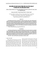
Figure 2. (a) Experimental and theoretical atomic hard-
nesses for main group elements. Plotted are the experi-
mental data and data obtained using eq 70 with C ) 0
(simplest) and C ) 0.499 eV (modified). (b) Experimental
and theoretical atomic hardnesses for transition elements.
Plotted are the experimental data and data obtained using
eq 70 with C ) 0 (simplest) and C ) 1.759 eV (modified).
Reprinted with permission from ref 174. Copyright 1997
American Chemical Society.
J )
∫∫
φ
1
*
(r
1
)φ
2
*
(r
2
)φ
1
(r
2
)φ
2
(r

2
)
|r
1
- r
2
|
dr
1
dr
2
≈ I - A
(73)
Table 1. Molecular Hardnesses (eV) As Calculated by
Different Methods
a
molecule (I - A)/2 (
L
- 
H
)/2 (η
+
+ η
-
)/2 η
+
η
-
BCl
3

6.537 7.294 1.566 1.561 1.570
BF
3
10.242 11.677 2.202 2.162 2.243
BH
3
7.192 7.973 2.285 2.041 2.530
C
2
H
2
7.610 8.509 2.088 1.983 2.192
C
2
H
4
6.549 7.569 1.864 1.820 1.909
C
2
H
6
9.501 9.943 1.649 1.428 1.871
CF
3
-
4.944 5.735 2.143 1.878 2.408
CF
3
+
9.576 11.388 2.466 2.516 2.416

CH
3
-
5.700 6.501 1.916 1.706 2.126
CH
3
+
8.021 9.071 2.574 2.256 2.892
CN
-
8.149 9.198 2.272 2.102 2.442
CNO
-
8.386 9.336 1.974 1.984 1.964
H
2
O 7.443 9.098 2.122 2.066 2.177
H
2
S 6.856 7.573 2.028 1.828 2.227
NCO
-
8.386 9.336 2.068 2.049 2.087
NH
2
-
5.958 7.098 2.060 1.918 2.202
NH
3
7.237 8.308 2.143 1.797 2.489

NH
4
+
12.021 12.851 2.150 1.735 2.566
PH
2
-
5.352 5.906 1.793 1.659 1.928
PH
3
5.746 6.331 1.900 1.733 2.068
PH
4
+
10.025 10.464 1.920 1.673 2.167
OH
-
6.761 8.176 2.441 2.345 2.537
HS
-
6.347 7.159 1.967 1.851 2.083
SO
2
6.224 7.012 2.012 1.977 2.046
SO
3
7.004 8.192 1.955 1.938 1.973
CO 8.579 9.715 2.684 2.373 2.994
H
2

CO 6.299 7.908 2.066 2.073 2.060
SCN
-
6.780 7.619 1.638 1.503 1.772
a
See text. Data from ref 150.
K )
∫∫
φ
1
*
(r
1
)φ
2
*
(r
2
)φ
1
(r
2
)φ
2
(r
1
)
|r
1
- r

2
|
dr
1
dr
2
(74)
η
ij
)
∂
2
E
∂n
i
n
j
(75)
η
ij
)
∂
i
∂n
j
(76)
η
ij
) [
i

(n
j
- ∆n
j
) - 
i
(n
j
)]/∆n
j
(77)
Conceptual Density Functional Theory Chemical Reviews, 2003, Vol. 103, No. 5 1805
to yield the total softness S and, from it, the total
hardness:
The results for a series of small molecules (HCN,
HSiN, N
2
H
2
, HCP, and O
3
H
+
) indicate, at first sight,
strong deviations between the HOMO-LUMO band
gap value and the η value obtained via the procedure
described above; introducing a factor of 2 (cf. eq 57)
brings the values relatively close to each other.
The evaluation of hardness in an atoms-in-mol-
ecules context (AIM) was reviewed by Nalewajski;

181
as further detailed in section III.B.3, the method is
based on the construction of a hardness tensor in an
atomic resolution, where the matrix elements η
ij
are
evaluated as will be explained here.
As in the MO ansatz described above, the global
hardness is then obtained via the softness matrix,
obtained after inverting η, summing its diagonal
elements, and inverting the total softness calculated
in that way:
An alternative and direct evaluation of the atomic
softness matrix, which can be considered as a gen-
eralization of the atom-atom polarizability matrix
in Hu¨ckel theory,
182
has been proposed by Cioslowski
and Martinov.
183
It should be noted that hardness can also be
obtained in the framework of the electronegativtity
equalization as described in detail by Baekelandt,
Mortier, and Schoonheydt.
184
The concept of hardness of an atom in a molecule
was also addressed by these and the present authors
by investigating the effect of deformation of the
electron cloud on the chemical hardness of atoms
(mimicked by placing fractions of positive and nega-

tive charges upon ionization onto neighboring atoms
and evaluating an AIM ionization energy or electron
affinity). The results generally point in the direction
of increasing hardness of atoms with respect to the
isolated atoms.
185
We end this section with a discussion of a reactivity
index combining electronegativity and hardness: the
electrophilicity index, recently introduced by Parr,
Von Szentpaly, and Liu.
186,187
These authors com-
mence by referring to a study by Maynard and co-
workers on ligand-binding phenomena in biochemical
systems (cf. section IV.C.2-f) involving partial charge
transfer,
188
where χ
2
A
/η
A
was first suggested as the
capacity of an electrophile to stabilize a covalent (soft)
interaction. They then addressed the question of to
what extent partial electron transfer between an
electron donor and an electron acceptor contributes
to the lowering of the total binding energy in the case
of maximal flow of electrons (note the difference with
the electron affinity measuring the capability of an

electron acceptor to accept precisely one electron).
Using a model of an electrophilic ligand immersed
in an idealized zero-temperature free electron sea of
zero chemical potential, the saturation point of the
ligand for electron inflow was characterized by put-
ting
For ∆E, the energy change to second order at fixed
external potential was taken,
where µ and η are the chemical potential and hard-
ness of the ligand, respectively.
If the electron sea provides enough electrons, the
ligand is saturated when (combining eqs 80 and 81)
which yields a stabilization energy,
which is always negative as η > 0. The quantity µ
2
/
2η, abbreviated as ω, was considered to be a measure
of the electrophilicity of the ligand:
Using the parabolic model for the E
ν
) E
ν
(N) curve
(eq 29), one easily obtains
and
The A dependence of ω is intuitively expected;
however, I makes the difference between ω and EA
(ω ∼ A if I ) 0), as there should be one as A reflects
the capability of accepting only one electron from the
environment, whereas ω is related to a maximal

electron flow.
Parr, Von Szentpaly, and Liu
186
calculated ω values
from experimental I and A data for 55 neutral atoms
and 45 small polyatomic molecules, the resulting ω
vs A plot illustrating the correlation (Figure 3).
ω values for some selected functional groups (CH
3
,
NH
2
,CF
3
, CCl
3
, CBr
3
, CHO, COOH, CN) mostly
parallel group electronegativity values with, e.g.,
ω(CF
3
) > ω(CCl
3
) > ω(CBr
3
), the ratio of the square
of µ and η apparently not being able to reverse some
electronegativity trends.
η )

1
S
)
1
∑
i
∑
j
S
ij
(78)
η
ij
f η f σ ) η
-1
f
∑
i
σ
ii
) S f η )
1
S
(79)
∆E/∆N ) 0 (80)
∆E ) µ∆N +
1
2
η∆N
2

(81)
∆N
max
)-
µ
η
(82)
∆E )-
µ
2
2η
(83)
ω )
µ
2
2η
(84)
∆N
max
) N
max
- N
0
)
1
2
I + A
I - A
(85)
ω )

(I + A)
2
8(I - A)
(86)
1806 Chemical Reviews, 2003, Vol. 103, No. 5 Geerlings et al.
Note, however, that ω(F) (8.44) > ω(Br) (7.28) .
ω(I) (6.92) > ω(Cl) (6.66 eV), where the interplay
between µ and η changes the electronegativity order,
F > Cl > Br > I, however putting Cl with lowest
electrophilicity.
3. The Electronic Fukui Function, Local Softness, and
Softness Kernel
The electronic Fukui function f(r), already pre-
sented in Scheme 4, was introduced by Parr and
Yang
189,190
as a generalization of Fukui’s frontier MO
concept
191-193
and plays a key role in linking frontier
MO theory and the HSAB principle.
194
It can be interpreted (cf. the use of Maxwell’s
relation in this scheme) either as the change of the
electron density F(r) at each point r when the total
number of electrons is changed or as the sensitivity
of a system’s chemical potential to an external
perturbation at a particular point r,
The latter point of view, by far the most prominent
in the literature, faces the N-discontinuity problem

of atoms and molecules,
89,90
leading to the introduc-
tion
189
of both right- and left-hand-side derivatives,
both to be considered at a given number of electrons,
N ) N
0
:
for a nucleophilic attack provoking an electron in-
crease in the system, and
for an electrophilic attack provoking an electron
decrease in the system.
The properties of the Fukui function have been
reviewed by Ayers and Levy:
190
besides normalization
and asymptotic decay, the cusp condition for the
density
195
implies that the Fukui function should also
satisfy it.
196
The essential role of the Fukui function in DFT has
recently been re-emphasized by Ayers and Parr,
197
stressing the point that the FF minimizes the hard-
ness functional η[F
N

0
,∆F
+1
], where ∆F
+1
stands for the
density distribution of the added electron subject to
the constraint that ∆F
+1
integrates to 1.
The importance of Fukui’s FMO concept in modern
chemistry can hardly be overestimated and is nicely
summarized in Kato’s perspective,
193
where it is said
that Fukui’s 1952 papers may be regarded as a bridge
connecting the two stages of chemical reactivity
description in the 20th century. The first stage is the
electronic theory of organic chemistry, generalized by
Coulson and Longuet-Higgins, based on quantum
mechanics. The second stage is the establishment of
symmetry rules for the MOs in predicting the course
of a reaction (i.e., FMO theory and Woodward-
Hoffmann rules). “Fukui’s paper proposed a reactivity
index for interpreting the orientation effect in a
chemical reaction, the main subject of the electronic
theory of organic chemistry, and was the starting
point of the second stage after the concept of frontier
orbitals was first introduced and it became the key
ingredient in the further development of the the-

ory.”
193
The electronic Fukui function now generalizes this
important concept.
Although, in principle, the neutral or N
0
-electron
system’s electron density contains all information
needed for the evaluation of the Fukui function, most
studies in the literature have been carried out in the
so-called finite difference method, approximating
Figure 3. Correlation between electrophilicity ω and electron affinity A for 54 atoms and 55 simple molecules. Reprinted
with permission from ref 186. Copyright 1999 American Chemical Society.
f(r) )
(
∂F(r)
∂N
)
ν
)
(
δµ
δν(r)
)
N
(87)
f
+
(r) )
(

∂F(r)
∂N
)
ν(r)
+
(88)
f
-
(r) )
(
∂F(r)
∂N
)
ν(r)
-
(89)
Conceptual Density Functional Theory Chemical Reviews, 2003, Vol. 103, No. 5 1807
and
which is, in many cases, seriously hampered by the
possibility of metastable anions.
124-126
A third function describing radical attack, f
0
(r), is
then obtained as the arithmetic average of f
+
(r) and
f
-
(r).

Note that, when a frozen approach is used when
studying the N
0
( 1 situations (e.g., describing them
with the orbitals of the N
0
system), f
+
(r) reduces to
F
LUMO
(r) and f
-
(r)toF
HOMO
(r), indicating that Fukui’s
frontier orbital densities can be considered as ap-
proximations to the function named in his honor.
192
Note also that Yang, Parr, and Pucci showed that f
+
and f
-
are directly related to the appropriate FMOs
198
and that f
+
(r) for an M-electron system may be
written as
and f

-
(r)as
in the context of Janak’s extension of Kohn-Sham
theory.
117
The earliest numerical calculations on Fukui func-
tions were reported by Lee, Yang, and Parr
199
(Figure
4), concentrating on the plots of the local softness
derived from it (vide infra) for H
2
CO, SCN
-
, and CO,
followed by studies by Mendez et al.
200,201
and Geer-
lings et al.
202-205
Particular attention to the (3D)
visualization of the Fukui function has been given
by Flurchick and Bartolotti.
206
When taken in com-
parative perspective, it was shown by the latter
authors that appreciable differences exist between
the HOMO (or LUMO) density and the Fukui func-
tion. Moreover, the suggestion by Gambiagi et al.
207,208

that f(r) is closely related to the Laplacian of the
charge density,
209,210
of fundamental importance in
Bader’s atoms-in-molecules theory,
68
turned out to be
not true. The influence of correlation on the Fukui
function was investigated by Langenaeker et al. in
the case of the f
-
(r) function of ambident nucleo-
philes (NO
2
-
,CH
2
CHO
-
, and SCN
-
), which showed
less important effects than expected. These studies
at a moderate level (CISD; 6-31++G**)
211
were later
completed by B3LYP-DFT and QCISD calculations
212
using Dunning’s augmented correlation-consistent
basis sets,

213,214
revealing for SCN
-
a slightly en-
hanced selectivity for the S-terminus in the case of
the DFT calculations, the QCISD and CISD results
being highly similar.
In recent years, intensive research has been con-
ducted on the development of methods avoiding the
rather cumbersome finite difference method, which
moreover bears sources of errors.
Figure 4. Parr’s early local softness plots for H
2
CO in the plane perpendicular to the molecular plane: nucleophilic vs
electrophilic reaction sites on H
2
CO, as indicated by s
+
(r) and s
-
(r), respectively. Reprinted with permission from ref 199.
Copyright 1988 Elsevier Science.
f
+
(r)asf
+
(r) ≈ F
N
0
+1

(r) -F
N
0
(r) (90)
f
-
(r)asf
-
(r) ≈ F
N
0
(r) -F
N
0-1
(r) (91)
f
+
(r) ) |Ψ
LUMO
(r)|
2
+
∑
i)1
M
∂
∂N
|Ψ
i
(r)|

2
(92)
f
-
(r) ) |Ψ
HOMO
(r)|
2
+
∑
i)1
M - 1
∂
∂N
|Ψ
i
(r)|
2
(93)
1808 Chemical Reviews, 2003, Vol. 103, No. 5 Geerlings et al.
A gradient approximation has been developed by
Chattaraj et al.
196
and Pacios et al.,
215,216
proposing
an expansion,
which was written as
where F
0

is the density at the nucleus, R being a
parameter which can be determined, e.g., from F
0
.
This technique, which was exclusively used for atoms
hitherto, yields a single Fukui function, not distin-
guishing between f
+
(r) and f
-
(r).
The results of the radial distribution of the Fukui
function, 4πr
2
f(r), for Li, N, and F are similar to those
obtained by Gazquez, Vela, and Galvan
217
using a
finite difference approach within a spin-polarized
formalism; they show a slow decay for electropositive
atoms and a faster one for electronegative atoms.
De Proft et al.
175
implemented the variational
principle for chemical hardness formulated by Chat-
taraj, Cedillo, and Parr,
172
stating that the global
hardness and the Fukui function can be obtained
simultaneously by minimizing the functional (69),

where η(r,r′) is the hardness kernel (see section
III.B.4) and where g(r) is constrained to integrate to
1. Whereas the gradient extension method does not
distinguish between f
+
(r) and f
-
(r), these functions
may be obtained in the variational approach by using
the one-sided hardness kernel, η
+
(r,r′)orη
-
(r,r′).
The extremal functional of eq 69 can be shown to
be the Fukui function, the functional η[g)f] leading
to the global hardness. As stated by Ayers and
Levy,
190
the variational method may be the method
of choice in the future, but the accurate determina-
tion of the hardness kernel remains a problem. This
conclusion also emerges in a natural way from the
recent in-depth and generalizing study by Ayers and
Parr on variational principles for describing chemical
reactions: the Fukui function appears as the function
minimizing the hardness functional.
197
Introducing the approximation
leads to the hardness expression

Using a linear combination of atomic Fukui functions,
the condensed form of this methodology was shown
to yield results in line with the sensitivity analysis
approach formulated by Nalewajski and was also
used by Mortier.
Nalewajski et al. showed that the Fukui function
can be obtained from a single Kohn-Sham calcula-
tion.
218
It is determined by adding to the rigid,
frontier orbital term (see also eqs 92 and 93) the
density relaxation contribution, which is determined
by differentiation of the Kohn-Sham equations with
respect to N:
Here, f
F
is the frontier term corresponding to the
“frozen” shape of orbitals, and f
R
corresponds to
orbital relaxation.
Neglecting the exchange correlation term in the N
derivative, contour maps of the Fukui function f
+
for
H
2
CO obtained in this analytical way (differential
Fukui Function) are compared in Figure 5 with the
finite difference results obtained with two different

∆N values, the usual |∆N| ) 1 case and a smaller
value (0.01), and with the LUMO density correspond-
ing to the first term in eq 95. It is seen that, as
compared to the LUMO density (antibonding π*
orbital), the orbital relaxation mixes the frontier
orbital with the other occupied MOs including σ
orbitals, a feature present in both the finite difference
and differential methods. In Figure 6, a more detailed
comparison between these two methods is given,
along a line parallel to the CO bond in the planes of
Figure 5. It is clearly seen that the differential
method approaches the finite difference results upon
decreasing ∆N. This trend is confirmed in other
cases.
217
Russo et al.
219
also presented an atoms-in-mol-
ecules variant of his MO approach, based on Mayer’s
Figure 5. f
+
contour diagram for H
2
CO in a plane
perpendicular to the molecular plane containing the CO
bond. Drawn are the differential f
+
(r), the finite diffence
f
+

(r) corresponding to ∆N ) 1 and ∆N ) 0.01, and the
LUMO density. Reprinted with permission from ref 218.
Copyright 1999 American Chemical Society.
f(r) ) f
F
(r) + f
R
(r) (98)
f(r) )
F(r)
N
[1 +RΦ(r,F(r),3F,3
2
F, )] (94)
f(r) )
F(r)
N
+
R
N
F
0
-2/3
{
[
(
F
F
0
)

2/3
- 1
]
3
2
F-
2
3
(
F
0
F
)
2/3
3F
0
‚3F
F
}
(95)
η(r,r′) ≈
1
|r - r′|
(96)
η )
∫∫
f(r) f(r′)
|r - r′|
dr dr′ (97)
Conceptual Density Functional Theory Chemical Reviews, 2003, Vol. 103, No. 5 1809

bond order indices and atomic valences.
220,221
A
similar approach was followed by Grigorov et al.,
using the thermal extension of DFT,
222,223
and by
Liu.
224
Landmark papers on the atoms-in-molecules
approach were written by Nalewajski et al., who
introduced these concepts in the late 1980s and early
1990s
225,226
(for reviews, see refs 227-229). It is one
of the most elaborated and documented techniques
to obtain information about Fukui functions and local
softness at the atomic level. It is, in fact, part of a
general analysis on intermolecular interactions in the
hardness/softness context. Depending on the resolu-
tion involved, specified by a given partitioning of the
system in the physical space, one defines the electron
density distribution F(r) (local resolution), the popu-
lation of atoms in molecules (N
A
, N
B
, etc.; AIM
resolution), the populations attributed to larger mo-
lecular fragments (e.g., groups; N

X
, N
Y
, N
Z
, etc.; group
resolution), or the total number of electrons (N )
∫F(r)dr ) ∑
A
N
A
) ∑
X
N
X
; global resolution). An
interesting intermediate resolution is situated at the
MO level.
230,231
In the AIM resolution, a semiempirical ansatz is
used to construct the elements of the atom-atom
hardness matrix, η
AB
, using the finite difference
formula, η
A
) (I
A
- A
A

)/2 (eq 56), for the diagonal
elements and the Ohno formula,
232,233
for the off-diagonal elements, R
AB
being the inter-
atomic distance, R
AB
being defined as
Note that Balawender and Komorowski
150
pre-
sented a coupled perturbed Hartree-Fock scheme
(for a comprehensive account of the CPHF methods,
see ref 133) in a MO basis to obtain first-order
correction terms to the orbital frozen Fukui function.
The matrix of the derivative MO coefficients
(∂C/∂N)
ν(r)
is written in terms of the unperturbed MOs
as eq 72, where U is determined via a coupled
perturbed Hartree-Fock scheme.
Retaining integer occupation numbers for the MOs
requires
The correlation between atomic Fukui function in-
dices obtained in this way and the finite difference
approximation turns out to be remarkably good in a
series of diatomics.
Russo and co-workers presented
52,219

a method
based on the diagonalization of the hardness matrix
in a valence MO basis, n
ij
) ∂
i
/∂n
j
, yielding orbital
Fukui functions, the Kohn-Sham eigenvalues 
i
being evaluated on the basis of Janak’s theorem.
117
Senet
234,235
proposed a different methodology based
on the knowledge of the linear response function
χ(r,r′), offering also a generalization to higher order
Fukui functions,
for which, however, no numerical results have been
reported yet.
Preceding Nalewajski’s AIM approach, a condensed
form of the Fukui function was introduced in 1986
by Yang and Mortier,
236
based on the idea of inte-
grating the Fukui function over atomic regions,
similar to the procedure followed in population
analysis techniques.
237

Combined with the finite
difference approximation, this yields working equa-
tions of the type
where q
A
(N) denotes the electronic population of atom
A of the reference system, more carefully denoted as
q
A,N
0
. The simplification of eq 103 in the frozen orbital
approach has been considered by Contreras et al.
238
Obviously, the q
A
values will be sensitive both to
the level of the calculation of the electron density
function F(r) which is differentiated and to the
partitioning scheme. As such, the inclusion of cor-
relation effects in the Hartree-Fock-based wave
function-type calculations is crucial, as is the choice
of the exchange correlation functional in DFT meth-
ods (cf. the change in the number of electron pairs
when passing from N
0
to N
0
+ 1orN
0
- 1).

Figure 6. Comparison between the finite difference and
differential f
+
results for H
2
CO along a line parallel to the
CO bond in the plane of the figure. Curve 1 is the
differential result; curves 2, 3, and 4 represent the finite
difference results with ∆N ) 0.01, 0.5, and 1.0, respectively.
Reprinted with permission from ref 218. Copyright 1999
American Chemical Society.
η
AB
) 1/

R
AB
2
+ R
AB
2
(99)
2
(η
A
+ η
B
)
(100)
f

+
)
(
∂n
i
∂N
)
+
) 0 i * LUMO
) 1 i ) LUMO
(101)
f
-
)
(
∂n
i
∂N
)
-
) 0 i * HOMO
) 1 i ) HOMO
(102)
(
∂
n
f(r)
∂N
n
)

ν(r)
)
(
∂
n+1
F(r)
∂N
n+1
)
ν(r)
(103)
f
A
+
) q
A
(N + 1) - q
A
(N) t q
A,N
0
+1
- q
A,N
0
(104)
f
A
-
) q

A
(N) - q
A
(N - 1) t q
A,N
0
+1
- q
A,N
0
-1
(105)
1810 Chemical Reviews, 2003, Vol. 103, No. 5 Geerlings et al.
The partitioning scheme encompasses the panoply
of techniques in population analysis, varying from
Mulliken,
239
over CHELPG
240
and natural population
analysis,
241
to Cioslowski’s atomic polar tensor (APT)-
based formalism
242-244
and Bader’s atoms-in-mol-
ecules picture.
68
Comprehensive studies, including
also the effect of the atomic orbital basis set, have

been performed by Martin, De Proft, and Geer-
lings,
56,212,245
Chermette and co-workers,
246
Aru-
mozhiraja and Kolandaivel,
247
and Cioslowski et al.
243
Taking QCISD
248,249
results as a reference, Geerlings
showed that B3LYP and especially B3PW91 perform
very well, better than Hartree-Fock and MP2 in
combination with NPA or Bader’s analysis, APT
being computationally demanding for larger systems,
since dipole moment derivatives are involved.
242
It
is the authors’ experience that problems of basis set
dependence of atomic populations are often trans-
ferred to condensed Fukui functions. Basis set and
population analysis sensitivity are still prominent in
the condensed FF values, as also noticed by Aru-
mozhiraja and Kolandaivel.
247
Chermette, on the
other hand, used a numerical integration scheme
derived by Becke,

250
dividing the three-dimensional
space into weighted atomic subregions. In an exten-
sive study on maleimide, a gratifying stability of the
f
A
values was found for various combinations of
exchange correlation functionals, basis sets, and also
for the numerical parameters defining the grid.
Most studies hitherto concentrated on condensed
Fukui functions for closed-shell molecules; studies
exclusively devoted to open-shell molecules are scarce.
Misra and Sannigrahi,
251
in a study of small radicals,
found this effect of spin contamination on the finite
difference Fukui function to be small. In a recent
study,
252
the DFT-B3LYP approach was preferred to
the use of UHF wave functions, as the latter are
appreciably spin-contaminated in many cases. Chan-
dra and Nguyen were the first to use Fukui functions
to study reactions involving the attack of radicals on
nonradical systems (in the case of olefins)
253
(see
section IV.C.2-d). Kar and Sannigrahi, on the other
hand,
252

used f
0
and s
0
values in the study of radical
reactions, concentrating on the stereoselectivity of
radical-radical interactions, invoking a HSAB-type
(section III.C.3) argument that sites of maximal f
0
should interact.
When working at the local level, eqs 104 and 105
sometimes lead to negative Fukui functions which,
at first sight, may seem contra-intuitive. However,
although this problem has been investigated in detail
by Roy et al.,
254,255
no definitive answer has been
given yet to the question of whether negative values
are physically acceptable or are artifacts. In the case
of the condensed Fukui function, Fuentealba et al.
256
presented a series of arguments for a positive definite
condensed Fukui function based on an analysis of the
finite difference expressions, eqs 104 and 105. Pos-
sible origins of negative Fukui functions have been
attributed by Roy et al. to relaxation effects and
improper charge partitioning techniques. A thorough
study on the nature of the Mulliken-based condensed
Fukui function indices indicates that, analytically,
nothing can be predicted about the sign of the

condensed Fukui function indices.
257
These authors promoted Hirshfeld’s stockholder
partitioning technique,
258,259
later discussed by Maslen
and Spackman
260
as a partitioning technique superior
to others (although it was remarked that there are
sites having negative values).
This technique has also been recently used by the
authors
261
in view of the recent information theory-
based proof by Parr and Nalewajski, which showed
that when maximal conservation of the information
content of isolated atoms is imposed upon molecule
formation, the stockholder partitioning of the electron
density is recovered.
262
It was seen that Hirshfeld
charges can be condensed as a valuable tool to
calculate Fukui function indices.
Moreover, Ayers
263
showed that Hirshfeld charges
also yield maximally transferable AIMs, pointing out
that the strict partitioning of a molecule into atomic
regions is generally inconsistent with the require-

ment of maximum transferability.
Nalewajski and Korchowiec
229,264-266
extended the
Fukui function concept to a two-reactant description
of the chemical reaction. A finite difference approach
to both diagonal and off-diagonal Fukui functions in
local and AIM resolutions was presented, considering
these functions as components of the charge-transfer
Fukui function, f
CT
(r):
where
and
with
In a case study on the reaction of a methyl radical
with ethylene, it was concluded that the reorganiza-
tion of electron density due to charge transfer is
proportional to the sum of forward (AB) and back-
ward (BA) f
CT
(r), involving both diagonal and off-
diagonal Fukui functions.
The Fukui function clearly contains relative infor-
mation about different regions in a given molecule.
When comparing different regions in different mol-
ecules, the local softness turns out to be more
interesting (for a review, see ref 49).
This quantity s(r) was introduced in 1985 by Yang
and Parr as

267
as a local analogue of the total softness S, which can
be written as
f
CT
(r) )
(
∂F(r)
∂N
CT
)
(106)
dN
CT
) dN
A
)-dN
B
(107)
f
CT
(r) ) {f
AA
(r) - f
BA
(r)} + {f
AB
(r) - f
BB
(r)}

(108)
f
AA
(r) )
(
∂F
A
(r)
∂N
A
)
f
AB
(r) )
(
∂F
A
(r)
∂N
B
)
(109)
s(r) )
(
∂F(r)
∂µ
)
ν(r)
(110)
Conceptual Density Functional Theory Chemical Reviews, 2003, Vol. 103, No. 5 1811

By applying the chain rule, s(r) can be written as
the product of the total softness and the Fukui
function,
indicating that f(r) redistributes the global softness
among the different parts of the molecule and that
s(r) integrates to S:
The predictive power for intermolecular reactivity
sequences of the local softness clearly emerges from
consideration of eq 110, showing that f(r) and s(r)
contain the same information on the relative site
reactivity within a single molecule, but that s(r), in
view of the information about the total molecular
softness, is more suited for intermolecular reactivity
sequences.
It is interesting to note that the concepts of
hardness and Fukui function (and thus also the local
softness) can be extended to the theory of metals.
267
It was shown by Yang and Parr that, at T ) 0,
and
where g(
F
) and g(
F
,r) are the density of states and
the local density of states at the Fermi level, respec-
tively. g() and g(,r) are defined respectively as
267,268
Methodological issues for the calculation of s(r) can
be brought back to those of f(r) and S in view of eq

112, and we refer to section III.B.3.
In fact, relatively few softness plots have been
shown in the literature, their discussion being almost
always devoted to the intramolecular reactivity se-
quences, for which f(r) can serve as well. Direct
applications are mostly reported in a condensed form
completely equivalent to the condensed Fukui func-
tion equations, e.g., in the finite difference approach:
A variety of techniques described for the Fukui
function have been used to calculate them. Recently,
a new approach was presented by Russo et al.,
obtaining AIM softnesses
218
from Mayer’s atomic
valences.
219,220
In recent years, to cope with the problem of
negative Fukui functions, Roy et al. introduced a
relative nucleophilicity and a relative electrophilicity
index defined as follows in atomic resolution.
269,270
For
an atom k, one writes
It was argued that the individual values of s
k
+
and s
k
-
might be influenced by basis set limitations and thus

insufficiently take into account electron correlation
effects.
Derivatives of the Fukui function or local softness
were scarcely considered in the literature. Parr,
Contreras, and co-workers
271,272
introduced (∂f/∂N)
ν
,
(∂f/∂µ)
ν
, and (∂s/∂N)
ν
.
One can expect, as argued by Fuentealba and
Cedillo,
273
that, e.g., a quantity of the type ∂f(r)/∂N
should be small. (It is exactly zero in the approxima-
tion f(r) ) 1/NF(r) used as the first order in the
gradient expansion.)
Of larger direct importance may be the variation
of the FF under an external perturbation, for which
some model calculations in the case of the H atom
perturbed by a proton or an electric field have been
reported by the same authors.
273
It should finally be noticed that Mermin
105
formu-

lated a finite temperature version of DFT in which
density and temperature define everything, even for
nonhomogeneous systems. In the grand canonical
ensemble, global and local softness are related to
density and number fluctuations,
267
with β ) 1/kT and where “〈〉” indicate averages over
the grand canonical ensemble.
Using the finite temperature version of DFT,
Galvan et al.
274
were able to establish an interesting
and promising relationship between the local soft-
ness, s(r), and the conductance in the context of
scanning tunneling microscopy (STM) images,
275,276
stressing the possibility of obtaining experimental
local softnesses for surfaces.
We finally consider the softness kernel, s(r,r′),
introduced by Berkowitz and Parr
277
and defined as
Here, u(r) is the modified potential,
Upon integration of s(r,r′), we obtain a quantity,
t(r),
s
k
-
/s
k

+
(relative nucleophilicity) and
s
k
+
/s
k
-
(relative electrophilicity)
S ) β[〈N
2
〉 - 〈N〉〈N〉] (120)
s(r) ) β[〈NF(r)〉 - 〈N〉〈F(r)〉] (121)
s(r,r′) )-
δF(r′)
δu(r)
)-
δF(r)
δu(r′)
(122)
u(r) ) ν(r) - µ )-
δF[F]
δF
(123)
t(r) )
∫
s(r,r′)dr′ (124)
S )
(
∂N

∂µ
)
ν(r)
(111)
s(r) )
(
∂F(r)
∂µ
)
ν
)
(
∂F(r)
∂N
)
ν
(
∂N
∂µ
)
ν
) Sf(r) (112)
∫
s(r)dr )
∫
Sf(r)dr ) S
∫
f(r)dr ) S (113)
1
η

) g(
F
) (114)
f(r) )
g(
F
,r)
g(
F
)
(115)
g() )
∑
i
δ(
i
- ) (116)
g(,r) )
∑
i
|Ψ
i
(r)|
2
δ(
i
- ) (117)
s
A
+

) s
A
(N + 1) - s
A
(N) t s
A,N
0
+1
- s
A,N
0
(118)
s
A
-
) s
A
(N) - s
A
(N - 1) t s
A,N
0
- s
A,N
0
-1
(119)
1812 Chemical Reviews, 2003, Vol. 103, No. 5 Geerlings et al.
which can be identified
189,277

as
and which couples the conventional linear response
function (δF(r)/δν(r′))
N
) χ
1
(r,r′) in Scheme 4 to the
softness kernel:
In the same spirit as eq 121, it has been shown
that the following fluctuation formula holds for the
softness kernel:
The corresponding hardness kernel, η(r,r′), defined
as (vide infra)
yields a reciprocity relation between η(r,r′) and
s(r,r′), in the sense that
Senet
234,235
showed that Fukui functions can be
related to the linear response function χ
1
(r,r′) through
the following equation:
Approximate expressions for the calculation of
the linear response function have been derived by
Fuentealba,
278
yielding, however, constant local hard-
ness η(r) (see section III.B.4)
Higher order response functions have been pro-
posed in the literature by Senet

234,235
and by Fuen-
tealba and Parr
271,273,279
with complete computational
schemes up to nth order. Numerical results, already
present for the first-order derivative of η with respect
to N (third-order energy derivative),
271
are still scarce.
It will be interesting to see whether, in the near
future, practical calculation schemes will be devel-
oped and what the order of magnitude of these
quantities will be determining their role in chemical
reactivity. The demand for visualization of these
quantities will also present a challenge. Recent
results by Toro-Labbe´ and co-workers for the hard-
ness derivatives of HCXYH (X, Y ) O, S) and their
hydrogen-bonded dimers indicated low γ values.
280
On the other hand, in a functional expansion
281
study
of the total energy, Parr and Liu
282
gave arguments
for a second-order truncation, stating that it is quite
natural to assume that third-order quantities of the
type δ
3

F/δF(r)δF(r′)δF(r′′) would be small and that the
quantities entering second-order formulas for chemi-
cal charges are “tried and true” ingredients of simple
theories.
4. Local Hardness and Hardness Kernel
The search for a local counterpart of η, the local
hardness
283
for which in this review the symbol η(r)
will be used throughout, turns out to be much more
complicated than the search for the global-local
softness relationship discussed in section III.B.3,
which resulted in an expression (eq 113) indicating
that the Fukui function distributes the global soft-
ness among the various parts of the system.
The search for a local counterpart of the hardness
begins by considering
Note that this quantity also appears in a natural way
when the chain rule is applied to the global hardness:
An explicit expression for η(r) can be obtained by
starting from the Euler equation (6) and multiplying
it by a composite function λ(F(r)),
284
integrating to N:
yielding
Taking the functional derivative with respect to F(r)
at fixed ν yields, after some algebra,
If one forces the local hardness into an expression
of type
which is desirable if a simple relationship with the

second functional derivative of the Hohenberg-Kohn
functional is the goal, then an additional constraint
for the composite function λ(F(r)) appears:
285
As the hardness kernel is defined as shown in eq
128,
189,283
the expression for local hardness then
becomes
The ambiguity in the definition of the local hard-
ness was discussed by Ghosh,
286
Harbola, Chattaraj,
and Parr,
284,287
Geerlings et al.,
285
and Gazquez.
173
Restricting λ to functions of the first degree in F, the
t(r) ) Sf(r) ) s(r) (125)
(
δF(r)
δν(r′)
)
N
)-s(r,r′) +
s(r)s(r′)
S
(126)

s(r,r′) )
1
kT
[〈F(r)F(r′)〉 - 〈F(r)〉〈F(r′)〉] (127)
η(r,r′) )
δ
2
F[F]
δF(r)δF(r′)
(128)
∫
s(r,r′)η(r′,r′′)dr′ ) δ(r - r′′) (129)
∫
χ
1
(r,r′)η(r′,r′′)dr′ ) f(r) - δ(r - r′′)
(130)
η(r) )
(
δµ
δF(r)
)
ν
(131)
η )
1
2
(
∂
2

E
∂N
2
)
ν
)
1
2
(
∂µ
∂Ν
)
ν
)
1
2
∫
(
δµ
δF(r)
)
ν
(
δF(r)
δN
)
ν
dr
)
1

2
∫
η(r) f(r)dr (132)
∫
λ(F(r)) dr ) N (133)
Nµ )
∫
ν(r)λ(F(r)) dr +
∫
δF
HK
δF(r)
λ(F(r)) dr
(134)
(
δµ
δF
)
ν
)
1
N
((
∂λ(F(r))
∂F(r)
)
- 1
)
µ +
1

N
∫
δ
2
F
HK
δF(r)δF(r′)
λ(F(r′)) dr′ (135)
(
δµ
δF
)
ν
)
1
N
∫
δ
2
F
HK
δF(r)δF(r′)
λ(F(r′)) dr′ (136)
(
∂λ(F(r))
∂F
)
ν
) 1 (137)
η

λ
(r) )
1
N
∫
η(r,r′)λ(F(r′)) dr′ (138)
Conceptual Density Functional Theory Chemical Reviews, 2003, Vol. 103, No. 5 1813
following possibilities emerge:
The latter case yields, however,
284,285
i.e., a local hardness equal to the global hardness at
every point in space. At first sight, this form is less
appropriate as (quoting Pearson
121
), “unlike the
chemical potential there is nothing in the concept of
hardness which prevents it from having different
values in the different parts of the molecule”. The
choice leading to η(r) ) η leads to the question of
whether we could not do without the local hardness
in DFT or if another quantity should be considered
to play this role. On the other hand, the result leads
to an increased emphasis on local softness and
attributes a smaller role to local hardness.
Parr and Yang
23
stated that the (δ
2
F/δF(r)δF(r′))
functional derivative, the hardness kernel η(r,r′), is

of utmost importance, as can be expected from the
second functional derivative of the universal Hohen-
berg-Kohn functional with respect to F(r), the basic
DFT quantity. It appears in a natural way when the
chain rule is applied to the global hardness:
It was shown
288
that, starting from the Thomas-
Fermi-Dirac approach and taking into account the
exponential fall-off of the density in the outer regions
(see also ref 285), η
D
(r) can be approximated as
V
el
(r) being the electronic part of the molecular
electrostatic potential
289
[for applications of these
working equations, see section IV.C.3].
It should be clear that, as opposed to the local
softness s(r), η(r) as seen in eq 132 does not integrate
to its global counterpart. Only upon multiplication
by the electronic Fukui function is η recovered upon
integration. This prompted an introduction of a
hardness density,
285
yielding, in the TFD approximation mentioned above,
the following working equations
Local hardness in the form η

D
(r) appears in a
natural way in the hardness functional,
introduced by Parr and Gazquez,
290
for which at all
orders
Let us finally come back to the hardness kernel
η(r,r′). It can be seen that the softness kernel s(r,r′)
and η(r,r′) are reciprocals in the sense that
Using eqs 124 and 125 and the local hardness
expression η
D
, one finds
indicating that s(r) and η
D
(r) are reciprocals, in the
sense that
The explicit form of the hardness kernel, in view
of its importance, has gained widespread interest in
the literature: Liu, De Proft, and Parr for example,
174
proposed for the expression
various approximation for R(r,r′), the 1/|r - r′|
arising from the classical Coulombic part in the
Hohenberg-Kohn universal density functional. Vari-
ous approaches to R(r,r′) were presented to take into
account the kinetic energy, exchange, and correlation
parts.
An extensive search for the modelization of the

hardness kernel at the AIM level (cf. section III.B.3)
has been carried out by Nalewajski, Mortier, and
others.
184,226,230,231,291-295
5. The Molecular Shape FunctionsSimilarity
The molecular shape function, or shape factor σ(r),
introduced by Parr and Bartolotti,
296
is defined as
λ(F(r)) )F(r) yielding
η
D
(r) )
1
N
∫
η(r,r′)F(r′)dr′ (139)
λ(F(r)) ) Νf(r) yielding
η
D
(r) )
∫
η(r,r′)f(r′)dr′ (140)
η
F
(r) ) η (141)
η )
1
2
(

∂
2
E
∂N
2
)
ν
)
1
2
∫∫
δ
2
F
HK
δF(r)δF(r′)
f(r)f(r′)dr dr′
(142)
η
D
(r) ≈ -
1
2N
V
el
(r) (143)
h(r) ) η
λ
(r)f(r) (144)
h

D
(r) ≈ -
1
4N
V
el
(r)f(r) (145)
h
F
(r) ≈
1
4N
(
∂V
el
(r)
∂N
)
ν(r)
F(r) (146)
H[F] )
∫
F(r)
δF[F]
δF(r)
dr - F[F] (147)
δH[F]
δF
) Nη
D

(r) (148)
∫
s(r,r′)η(r′,r′′)dr′ ) δ(r - r′′) (149)
∫
s(r)η
D
(r)dr
)
∫
s(r,r′)dr′
1
N
∫
η(r,r′′)F(r′′)dr′′ dr
)
∫
F(r′′)dr′′ dr′
1
N
∫
s(r,r′)η(r,r′′)dr
)
1
N
∫
F(r′′)dr′′ dr′δ(r - r′′)
)
1
N
∫

F(r)dr ) 1 (150)
∫
s(r)η
D
(r)dr ) 1 (151)
η(r,r′) )
1
|r - r′|
+R(r,r′) (152)
σ(r) )
F(r)
N
(153)
1814 Chemical Reviews, 2003, Vol. 103, No. 5 Geerlings et al.
It characterizes the shape of the electron distribution
and carries relative information about this electron
distribution. Just as the electronic Fukui function
redistributes the (total) softness over the various
parts of the molecule (eq 112), σ(r) redistributes the
total number of electrons.
Just as f(r), σ(r) is normalized to 1:
N and σ(r) are independent variables, forming the
basis of the so-called isomorphic ensemble.
297
(Re-
cently, however Ayers argued that, for a finite
Coulombic system, σ(r) determines both ν(r) (as F(r)
does) and N.
298
)

Baekelandt, Cedillo, and Parr
299,300
showed that the
hardness in the canonical ensemble, η
ν
(the η expres-
sion, eq 57, used in this review hitherto), and its
counterpart in the isomorphic ensemble, η
σ
, are
related via the following equation:
where it is easily seen that
a fluctuation term involving the deviation of the
Fukui function from the average electron density per
electron.
The (δµ/δσ(r))
N
index was identified as a nuclear/
geometrical reactivity index related to local hardness
(cf. section III.B.4):
with
De Proft, Liu, and Parr provided an alternative
definition for the local hardness in this ensemble.
301
De Proft and Geerlings
302
concentrated on the
electronegativity analogue of eq 156,
pointing out that the electronegativity conventionally
used, χ

ν
, can be seen as a term representing the
energy versus N variation at fixed shape and a
contribution due to the variation of the energy with
the shape factor at a fixed number of electrons
modulated by a fluctuation term. The quantity
(δE/δσ(r))
N
can be put on equal footing with the first-
order response functions in Scheme 4 (δE/δν(r))
N
()F(r)) and (∂E/∂N)
ν
()-χ).
A possible way to model changes in the shape factor
is to substitute a particular orbital, Ψ
i
, in the density
expression by a different one, Ψ
j
. Working within a
Hartree-Fock scheme and using a Koopmans type
of approximation, one gets
Identifying Ψ
i
and Ψ
j
with Ψ
HOMO
and Ψ

LUMO
, and
using the approximation of eq 68 for the hardness,
we obtain
indicating that polarizable systems (η large, R small;
cf. section IV.A) show a higher tendency to change
their shape factor. A similar conclusion was reached
by Fuentealba.
303
We finally mention that Chan and Handy
304
intro-
duced the shape factor for subsystems, with density
F
i
(r) satisfying the relation
with
n
i
being the subsystem’s occupation numbers, the
total number of subsystems being m. The concept of
electronic chemical potential was extended to the
shape chemical potential of the subsystem i,
the indices indicating that the occupation numbers
of all subsystems different from i and the shape
functions of all subsystems are held fixed. It was
proven that, as opposed to µ (eq 37), the µ
i
values in
eq 166 do not equalize between subsystems, the

advantage being that this property characterizes the
electron-attracting/-donating power of any given den-
sity fragment rather than that of the system as a
whole.
The importance of the shape factor is also stressed
in a recent contribution by Gal,
305
considering dif-
ferentiation of density functionals A[F] conserving the
normalization of the density. In this work, functional
derivatives of A[F] with respect to F are written as a
sum of functional derivatives with respect to F at
fixed shape factor σ,“δ
σ
F”, and fixed N,“δ
N
F”,
respectively:
The shape factor σ(r) plays a decisive role when
comparing charge distributions and reactivity be-
tween molecules. In this context, the concept of
F(r) ) Nσ(r) (154)
∫
σ(r)dr ) 1 (155)
η
ν
) η
σ
+
∫

(
δµ
δσ(r)
)
N
(
∂σ(r)
∂N
)
ν
dr (156)
(
∂σ(r)
∂N
)
N
)
1
N
(f(r) - σ(r)) (157)
η
ν
)
∫
h(r)f(r)dr η
σ
)
∫
h(r)σ(r)dr (158)
h(r) )

1
N
(
δµ
δσ(r)
)
N
(159)
χ
ν
) χ
σ
+
∫
(
δE
δσ(r)
)
N
(
dσ(r)
dN
)
ν
dr (160)
(
∆E
∆σ(r)
)
N

≈

j
- 
i
|Ψ
j
(r)|
2
- |Ψ
i
(r)|
2
N (161)
F)
∑
i
n
i
|φ
i
|
2
(162)
(
∆E
∆σ(r)
)
N
≈ N

η
|Ψ
LUMO
(r)|
2
- |Ψ
HOMO
(r)|
2
(163)
F(r) )
∑
i
m
F
i
(r) (164)
F
i
(r) ) n
i
σ
i
(r) (165)
µ
i
)
(
∂E
∂n

i
)
n
j
,σ
i
(166)
δA[F]
δF(r)
)
δA[F]
δ
σ
F(r)
+
δA[F]
δ
N
F(r)
(167)
Conceptual Density Functional Theory Chemical Reviews, 2003, Vol. 103, No. 5 1815
“similarity” of charge distributions has received
considerable attention in the past two decades, under
the impetus of R. Carbo and co-workers (for reviews
see, for example, refs 306-309).
Several similarity indices have been proposed for
the quantum molecular similarity (QMS) between
two molecules, A and B, of which the simplest form
is written as
310

Introducing the shape factor σ(r) via eq 154, this
expression simplifies to
indicating that the similarity index depends only on
the shape of the density distribution and not on its
extent. The latter feature emerges in the so-called
Hodgkin-Richards
311
index,
which, upon introduction of the shape factor, reduces
to
which cannot be simplified for the number of elec-
trons of the molecules A and B (N
A
, N
B
). Both the
shape and the extent (via N) of the charge distribu-
tion are accounted for in the final expression.
To yield a more reactivity-related similarity index,
Boon et al.
312
proposed to replace the electron density
in eq 168 by the local softness, s(r), yielding a Carbo-
type index:
Exploiting the analogy between σ(r) and f(r) (re-
distribution of the total number of electrons or the
total softness among various parts of space), eq 172
yields
This expression, in analogy with eq 169, depends
only on the Fukui function of the molecules A and

B, but not on their total softnesses, S
A
and S
B
. The
Hodgkin-Richards analogue of Z
AB
S
still combines
this information:
The quality of these various quantum similarity
descriptors has been studied systematically for a
series of peptide isosteres.
312,313
Isosteric replacement
of a peptide bond, sCOsNHs, has indeed been an
attractive strategy for circumventing the well-known
susceptibility of peptide bonds to hydrolysis.
314,315
In
the model system CH
3
sCOsNHsCH
3
, the sCOs
NHs moiety has been replaced by sCHdHs, sCFd
CHs (Z and E isomers), sCH
2
sCH
2

s, sCH
2
sSs,
sCOsCH
2
s, sCH
2
sNHs, sCCldCHs, etc., and
the merits of the various analogues have been
investigated.
In the first series of results obtained via numerical
integration of ∫F
A
(r)F
B
(r)dr and ∫s
A
(r)s
B
(r)dr, the
problem of the dependence of these integrals on the
relative orientation and position (besides conforma-
tional aspects) was avoided by aligning the central
bonds of the isosteres and bringing the centers of the
central bond to coincidence. For the softness similar-
ity, the (Z)-fluorinated alkene structure shows the
higher resemblance with the amide bond, due to the
similarity in polarity with the carbonyl group, in
agreement with the experimental results
316,317

on the
potential use of CdCsF as a peptidomimetic.
In a later study,
313
the problems of relative orienta-
tion and position were circumvented by introducing
the autocorrelation function,
318,319
first introduced in
molecular modeling and quantitative structure-
activity relationship studies by Moreau and Bro-
to,
320,321
and a principal component analysis,
322,323
moreover bringing butanone to the forefront, rather
than the (Z)-fluoroalkene structure.
6. The Nuclear Fukui Function and Its Derivatives
As seen in section III.B.3, the electronic Fukui
function comprises the response of a system’s electron
density function F(r) to a perturbation of its total
number of electrons N at a fixed external potential.
As such, it is part of the tree of response functions
in the canonical ensemble with the energy functional
E ) E[N,ν(r)].
The question of what would be the response of the
nuclei (i.e., their position) to a perturbation in the
total number of electrons is both intriguing and
highly important from a chemical point of view:
chemical reactions indeed involve changes in nuclear

configurations, and the relationship between changes
in electron density and changes in nuclear configu-
ration was looked at extensively by Nakatsuji in the
mid-1970s,
324-326
referring to the early work by
Berlin.
327
A treatment in complete analogy with the previous
paragraphs, however, leads to serious difficulties, as
a response kernel is needed to convert electron
density changes in external potential changes.
299,328
Cohen et al.
329,330
circumvented this problem by
introducing the nuclear Fukui function Φ
R
,
Z
AB
F
)
∫
F
A
(r)F
B
(r)dr
[

∫
F
A
2
(r)dr
∫
F
B
2
(r)dr]
1/2
(168)
Z
AB
F
)
∫
σ
A
(r)σ
B
(r)dr
[
∫
σ
A
2
(r)dr
∫
σ

B
2
(r)dr]
1/2
(169)
H
AB
F
)
2
∫
F
A
(r)F
B
(r)dr
∫
F
A
2
(r)dr +
∫
F
B
2
(r)dr
(170)
H
AB
F

)
2N
A
N
B
∫
σ
A
(r)σ
B
(r)dr
N
A
2
∫
σ
A
2
(r)dr + N
B
2
∫
σ
B
2
(r)dr
(171)
Z
AB
s

)
∫
s
A
(r)s
B
(r)dr
[
∫
s
A
2
(r)dr
∫
s
B
2
(r)dr]
1/2
(172)
Z
AB
s
)
∫
f
A
(r)f
B
(r)dr

[
∫
f
A
2
(r)dr
∫
f
B
2
(r)dr]
1/2
(173)
H
AB
S
)
2S
A
S
B
∫
f
A
(r)f
B
(r)dr
S
A
2

∫
f
A
2
(r)dr + S
B
2
∫
f
B
2
(r)dr
(174)
Φ
R
)
(
∂F
R
∂N
)
ν
(175)
1816 Chemical Reviews, 2003, Vol. 103, No. 5 Geerlings et al.
where F
R
is the force acting on the nucleus R, Φ
R
measuring its change when the number of electrons
is varied. This function does not measure the actual

response of the external potential to changes in N,
but rather the magnitude of the onset of the pertur-
bation (force inducing the displacement), and as such
is rewarding and reflects the electron-cloud preceding
idea present in “chemical thinking” on reactions.
331
Using a Maxwell-type relation, as in Schemes 4
and 5, Baekelandt
332
showed that Φ
R
also represents
the change of the electronic chemical potential upon
nuclear displacement R
R
:
In this way, a scheme in analogy with Scheme 4 can
be constructed starting from an E ) E[N,R
R
] rela-
tionship, the corresponding first-order response func-
tions being
and
the charge of the nuclei being fixed.
Only a relatively small number of studies have
been devoted to the NFF until now; the first numer-
ical results were reported only in 1998,
110
obtained
using a finite difference approach (vide infra) for a

series of diatomic molecules. In recent work by
Balawender and Geerlings, an analytical approach
was developed
333
in analogy with Komorowski and
Balawender’s coupled Hartree-Fock approach to the
electronic Fukui function,
150
previously applied in the
study of aromaticity (vide infra).
334
The results were compared with those of the finite
field approach for both (∂F
R
/∂N)
ν
and (∂µ/∂R
R
)
ν
.A
reasoning along the lines described in section III.B.2
for the analytical evaluation of η yields, after some
tedious matrix algebra, the expression
where the matrix f represents the derivative of the
MO occupation numbers when the total number of
electrons is unchanged. U
N
is defined as in eq 72. F
R

and S
R
are core and skeleton derivatives.
133
In the
case of S
R
, e.g., this becomes
where C is defined as in eq 72, and S
AO
denotes the
matrix of the overlap integrals in the atomic basis.
The G
N
matrix arises from the differentiation of the
two-electron part of the energy.
The solution of the U
N
matrix elements is obtained
via the coupled perturbed Hartree-Fock equations
for a single-configuration, closed-shell system.
133
It turns out that the correlation coefficient between
analytical and finite difference NFF is remarkably
high, both for the finite difference approach to
and for
In the former expression, µ has been approximated
by the FMO energy. The corresponding equations for
the left-side derivative are
As an example, we give in Table 2 the values of

the analytical NFF, ∇
R
E(N - 1), and ∇
R
e
HOMO
and
show in Figure 7a the correlation between the two
numerical approaches and in Figure 7b the correla-
tion between the analytical approach and ∇
R
e
HOMO
.
Molecules in the upper right quadrant show, in both
approaches, bond contraction upon ionization, whereas
those in the lower left quadrant show bond elonga-
tion.
The analytical results can be interpreted in terms
of the Hellman-Feynman theorem
335,336
for the force
F
R
acting on nucleus R:
Φ
R
)
(
∂F

R
∂N
)
ν
)
(
∂
2
E
∂R
R
∂N
)
ν
)
∂
∂R
R
(
∂E
∂N
)
ν
)
(
∂µ
∂R
R
)
N

(176)
(
∂E
∂R
R
)
N
)-F
R
(177)
(
∂E
∂N
)
R
R
) µ (178)
Φ
R
)-tr F
R
(f + U
N
n - nU
N
) +
tr S
R
(G
N

n + F(f + U
N
n - nU
N
)) (179)
S
R
) C
+
(
∂S
AO
∂R
R
)
C (180)
Table 2. Analytical Values of the Left Nuclear Fukui
Function (NFF “l”), Gradient of the Cation, and the
HOMO Energy for a Series of Diatomic Molecules
a
molecule NFF “l” HOMO gradient cation
AlCl 0.03625 0.04251 0.04277
AlF 0.04315 0.04469 0.04487
AlH 0.01437 0.01559 0.01129
BCl 0.05628 0.06623 0.07571
BeO -0.09816 -0.08233 -0.11307
BF 0.04559 0.07005 0.07182
BH 0.01171 0.01550 0.01689
Cl
2

0.05106 0.05548 0.05865
ClF 0.05145 0.07275 0.05410
CO 0.04578 0.06747 0.04114
CS -0.12344 -0.10465
F
2
0.09626 0.11894 0.12771
H
2
-0.16247 -0.16336 -0.14694
HCl -0.01470 -0.01194 -0.02144
HF -0.05530 -0.05540 -0.08623
Li
2
-0.00816 -0.00998 -0.00831
LiCl -0.03680 -0.03219 -0.03683
LiF -0.05649 -0.05545 -0.06650
LiH -0.02747 -0.02904 -0.02947
N
2
-0.04472 -0.05363 -0.04167
PN -0.13527 -0.11459 -0.06227
SiO 0.00110 0.01599 -0.06770
SiS -0.07833 -0.08475
a
Data from ref 60. All values are in au. Blank entries
correspond to cases where the highest occupied molecular
orbitals change their ordering upon increasing bond length.
(
∂F

R
∂N
)
ν
: Φ
R
+
) F
R
(N + 1) - F
R
(N) )-3
R
E(N + 1)
(181)
(
∂µ
∂R
R
)
N
: Φ
R
+
) 3
R
µ )-3
R
e
LUMO

(182)
Φ
R
-
)-3
R
E(N - 1) and Φ
R
-
)-3
R
e
HOMO
(183)
Conceptual Density Functional Theory Chemical Reviews, 2003, Vol. 103, No. 5 1817