Clarke f h , nonsmooth analysis and control theory (springer verlag, new york, 1998)

Graduate Texts
in
Mathematics
178
Editorial Board
S.
Axler
F.W.
Gehring
K.A.
Ribet
Springer
New
York
Berlin
Heidelberg
Barcelona
Budapest
Hong Kong
London
Milan
Paris
Santa Clara
Singapore
Tokyo
Graduate Texts
in
Mathematics
1
TAKEUTI/ZARING.

Introduction to
Axiomatic
Set
Theory.
2nd ed.
2 OxTOBY. Measure
and
Category.
2nd ed.
3 ScHAEFER. Topological Vector Spaces.
4
HILTON/STAMMBACH.
A Course in
Homological Algebra.
2nd ed.
5
MAC
LANE.
Categories
for the
Working
Mathematician.
6
HUGHES/PIPER.
Projective Planes.
7
SERRE.
A
Course
in

Arithmetic.
8
TAKEUTI/ZARING.
Axiomatic
Set
Theory.
9
HUMPHREYS.
Introduction
to Lie
Algebras
and Representation Theory.
10
COHEN.
A
Course
in
Simple Homotopy
Theory.
11
CONWAY.
Functions
of
One Complex
Variable
1. 2nd ed.
12
BEALS.
Advanced Mathematical Analysis.
13

ANDERSON/FULLER.
Rings
and
Categories
of Modules.
2nd ed.
14
GOLUBITSKY/GUILLBMIN.
Stable Mappings
and Their Singularities.
15
BERBERIAN.
Lectures
in
Functional
Analysis
and
Operator Theory.
16
WINTER.
The
Structure
of
Fields.
17
ROSENBLATT.
Random Processes.
2nd ed.
18
HALMOS.

Measure Theory.
19
HALMOS.
A
Hilbert Space Problem Book.
2nd
ed.
20
HUSEMOLLER.
Fibre Bundles.
3rd ed.
21
HUMPHREYS.
Linear Algebraic Groups.
22
BARNES/MACK.
An
Algebraic Introduction
to Mathematical Logic.
23
GREUB.
Linear Algebra.
4th ed.
24
HOLMES.
Geometric Functional Analysis
and
Its
Applications.
25

HEWITT/STROM BERG.
Real and Abstract
Analysis.
26
MANES.
Algebraic Theories.
27
KELLEY.
General Topology.
28
ZARISKI/SAMUEL.
Commutative Algebra.
Vol.1.
29
ZARISKI/SAMUEL.
Commutative Algebra.
Vol.11.
30
JACOBSON.
Lectures
in
Abstract Algebra
I.
Basic Concepts.
31
JACOBSON.
Lectures
in
Abstract Algebra
II.

Linear Algebra.
32
JACOBSON.
Lectures
in
Abstract Algebra
III.
Theory
of
Fields
and
Galois Theory.
33
HIRSCH.
Differential Topology.
34
SPITZER.
Principles
of
Random Walk.
2nd
ed.
35
ALEXANDER/WERMER.
Several Complex
Variables
and
Banach Algebras.
3rd ed.
36

KELLEY/NAMIOKA
et al. Linear
Topological Spaces.
37
MONK.
Mathematical Logic.
38
GRAUERT/FRITZSCHE.
Several Complex
Variables.
39
ARVESON.
An
Invitation
to
C*-Algebras.
40
KEMENY/SNELIVKNAPP.
Denumerable
Markov Chains.
2nd ed.
41
APOSTOL.
Modular Functions
and
Dirichlet Series
in
Number Theory.
2nd
ed.

42
SERRE.
Linear Representations
of
Finite
Groups.
43
GILLMAN/JERISON.
Rings
of
Continuous
Functions.
44
KENDIG.
Elementary Algebraic Geometry.
45
LOEVE.
Probability Theory
I. 4th ed.
46
LOEVE.
Probability Theory
II. 4th ed.
47
MOISE.
Geometric Topology
in
Dimensions
2 and 3.
48

SACHS/WU.
General Relativity
for
Mathematicians.
49
GRUENBERG/WEIR.
Linear Geometry.
2nd
ed.
50
EDWARDS.
Fermal's Last Theorem.
51
KLINGENBERG.
A
Course
in
Differential
Geometry.
52
HARTSHORNE.
Algebraic Geometry.
53
MANIN.
A
Course
in
Mathematical Logic.
54
GRAVER/WATKINS.

Combinatorics with
Emphasis
on the
Theory
of
Graphs.
55
BROWN/PEARCY.
Introduction
to
Operator
Theory
I:
Elements
of
Functional
Analysis.
56
MASSEY.
Algebraic Topology:
An
Introduction.
57
CROWELL/FOX.
Introduction
to
Knot
Theory.
58 KoBLiTZ. p-adic Numbers, p-adic
Analysis,

and
Zeta-Functions.
2nd ed.
59
LANG.
Cyclotomic Fields.
60
ARNOLD.
Mathematical Methods
in
Classical Mechanics.
2nd ed.
continued after index
EH.
Clarke
Yu.S.
Ledyaev
RJ. Stem
RR. Wolenski
Nonsmooth Analysis and
Control Theory
Springer
F.H. Clarke
Institut Desargues
Universit6 de Lyon I
Villeurbanne, 69622
France
R.J. Stem
JDepartment of Mathematics
Concordia University

7141 Sherbrooke St. West
Montreal, PQ H4B 1R6
Canada
Editorial Board
S. Axler
Mathematics Department
San Francisco State
University
San Francisco, CA 94132
USA
Yu.S.
Ledyaev
Steklov Mathematics Institute
Moscow, 117966
Russia
RR. Wolenski
Department of Mathematics
Louisiana State University
Baton Rouge, LA 70803-0001
USA
F.
W. Gehring
Mathematics Department
East Hall
University of Michigan
Ann Arbor, MI 48109
USA
K.A. Ribet
Department of Mathematics
University of California

at Berkeley
Berkeley, CA 94720-3840
USA
Mathematics Subject Classification (1991): 49J52,58C20,90C48
With
8
figures.
Library of
Congress
Cataloging-in-Publication Data
Nonsmooth analysis and control theory /
F.H.
Clarke . .
p.
cm. - (Graduate texts in mathematics ;
Includes bibliographical references and index.
ISBN
0-387-98336-8
(hardcover
:
alk. paper)
1.
Control Theory. 2. Nonsmooth optimization.
QA402.3.N66 1998
515'.64-dc21
.
[etal.].
178)
I. Clarke, Francis H. II. Series.
97-34140

©1998 Springer-Verlag New
York,
Inc.
All rights reserved. This work may not
be
translated or copied in whole or in part without the written
permission of
the
publisher (Springer-Verlag
New
York,
Inc.,
175
Fifth
Avenue,
New
York,
NY
10010,
USA),
except for brief excerpts in connection with reviews or scholarly analysis. Use in connection
with any form of information storage and rettieval, electronic adaptation, computer software, or by
similar or dissimilar methodology now known or hereafter developed is forbidden.
The use of general descriptive names, trade names, trademarks, etc., in this publication, even if the
former
are
not especially identified, is not to be taken as a sign that such
names,
as understood by the
Trade Marks and Merchandise

Marks
Act,
may accordingly be used freely by anyone.
ISBN
0-387-98336-8
Springer-Veriag New York Berlin Heidelberg SPIN 10557384
The authors dedicate this book:
to Gail, Julia, and Danielle;
to Sofia, Simeon, and Irina;
to Judy, Adam, and Sach; and
to Mary and Anna.
Preface
Pardon me for writing such a long letter; I had not the time to write a short
one.
—Lord Chesterfield
Nonsmooth analysis refers to differential analysis in the absence of differ-
entiability. It can be regarded as a subfield of that vast subject known as
nonlinear analysis. While nonsmooth analysis has classical roots (we claim
to have traced its lineage back to Dini), it is only in the last decades that
the subject has grown rapidly. To the point, in fact, that further devel-
opment has sometimes appeared in danger of being stymied, due to the
plethora of definitions and unclearly related theories.
One reason for the growth of the subject has been, without a doubt, the
recognition that nondifferentiable phenomena are more widespread, and
play a more important role, than had been thought. Philosophically at
least, this is in keeping with the coming to the fore of several other types
of irregular and nonlinear behavior: catastrophes, fractals, and chaos.
In recent years, nonsmooth analysis has come to play a role in functional
analysis, optimization, optimal design, mechanics and plasticity, differen-
tial equations (as in the theory of viscosity solutions), control theory, and,

increasingly, in analysis generally (critical point theory, inequalities, fixed
point theory, variational methods ). In the long run, we expect its meth-
ods and basic constructs to be viewed as a natural part of differential
analysis.
viii Preface
We have found that it would be relatively easy to write a very long book
on nonsmooth analysis and its applications; several times, we did. We have
now managed not to do so, and in fact our principal claim for this work is
that it presents the essentials of the subject clearly and succinctly, together
with some of its applications and a generous supply of interesting exercises.
We have also incorporated in the text a number of new results which clarify
the relationships between the different schools of thought in the subject.
We hope that this will help make nonsmooth analysis accessible to a wider
audience. In this spirit, the book is written so as to be used by anyone who
has taken a course in functional analysis.
We now proceed to discuss the contents. Chapter 0 is an Introduction in
which we allow ourselves a certain amount of hand-waving. The intent is
to give the reader an avant-goˆut of what is to come, and to indicate at an
early stage why the subject is of interest.
There are many exercises in Chapters 1 to 4, and we recommend (to the
active reader) that they be done. Our experience in teaching this material
has had a great influence on the writing of this book, and indicates that
comprehension is proportional to the exercises done. The end-of-chapter
problems also offer scope for deeper understanding. We feel no guilt in
calling upon the results of exercises later as needed.
Chapter 1, on proximal analysis, should be done carefully by every reader
of this book. We have chosen to work here in a Hilbert space, although the
greater generality of certain Banach spaces having smooth norms would be
another suitable context. We believe the Hilbert space setting makes for
a more accessible theory on first exposure, while being quite adequate for

later applications.
Chapter 2 is devoted to the theory of generalized gradients, which consti-
tutes the other main approach (other than proximal) to developing non-
smooth analysis. The natural habitat of this theory is Banach space, which
is the choice made. The relationship between these two principal approaches
is now well understood, and is clearly delineated here. As for the preceding
chapter, the treatment is not encyclopedic, but covers the important ideas.
In Chapter 3 we develop certain special topics, the first of which is value
function analysis for constrained optimization. This topic is previewed in
Chapter 0, and §3.1 is helpful, though not essential, in understanding cer-
tain proofs in the latter part of Chapter 4. The next topic, mean value
inequalities, offers a glimpse of more advanced calculus. It also serves as
a basis for the solvability results of the next section, which features the
Graves–Lyusternik Theorem and the Lipschitz Inverse Function Theorem.
Section 3.4 is a brief look at a third route to nonsmooth calculus, one that
bases itself upon directional subderivates. It is shown that the salient points
of this theory can be derived from the earlier results. We also present here
a self-contained proof of Rademacher’s Theorem. In §3.5 we develop some
Preface ix
machinery that is used in the following chapter, notably measurable selec-
tion. We take a quick look at variational functionals, but by-and-large, the
calculus of variations has been omitted. The final section of the chapter
examines in more detail some questions related to tangency.
Chapter 4, as its title implies, is a self-contained introduction to the theory
of control of ordinary differential equations. This is a biased introduction,
since one of its avowed goals is to demonstrate virtually all of the preceding
theory in action. It makes no attempt to address issues of modeling or
of implementation. Nonetheless, most of the central issues in control are
studied, and we believe that any serious student of mathematical control
theory will find it essential to have a grasp of the tools that are developed

here via nonsmooth analysis: invariance, viability, trajectory monotonicity,
viscosity solutions, discontinuous feedback, and Hamiltonian inclusions. We
believe that the unified and geometrically motivated approach presented
here for the first time has merits that will continue to make themselves felt
in the subject.
We now make some suggestions for the reader who does not have the time
to cover all of the material in this book. If control theory is of less interest,
then Chapters 1 and 2, together with as much of Chapter 3 as time al-
lows, constitutes a good introduction to nonsmooth analysis. At the other
extreme is the reader who wishes to do Chapter 4 virtually in its entirety.
In that case, a jump to Chapter 4 directly after Chapter 1 is feasible; only
occasional references to material in Chapters 2 and 3 is made, up to §4.8,
and in such a way that the reader can refer back without difficulty. The
two final sections of Chapter 4 have a greater dependence on Chapter 2,
but can still be covered if the reader will admit the proofs of the theorems.
A word on numbering. All items are numbered in sequence within a section;
thus Exercise 7.2 precedes Theorem 7.3, which is followed by Corollary 7.4.
For references between two chapters, an extra initial digit refers to the
chapter number. Thus a result that would be referred to as Theorem 7.3
within Chapter 1 would be invoked as Theorem 1.7.3 from within Chap-
ter 4. All equation numbers are simple, as in (3), and start again at (1) at
the beginning of each section (thus their effect is only local). A reference
to §3 is to the third section of the current chapter, while §2.3 refers to the
third section of Chapter 2.
A summary of our notational conventions is given in §0.5, and a Symbol
Glossary appears in the Notes and Comments at the end of the book.
We would like to express our gratitude to the personnel of the Centre
de Recherches Math´ematiques (CRM) of l’Universit´e de Montr´eal, and in
particular to Louise Letendre, for their invaluable help in producing this
book.

x Preface
Finally, we learned as the book was going to press, of the death of our
friend and colleague Andrei Subbotin. We wish to express our sadness at
his passing, and our appreciation of his many contributions to our subject.
Francis Clarke, Lyon
Yuri Ledyaev, Moscow
Ron Stern, Montr´eal
Peter Wolenski, Baton Rouge
May 1997
Contents
Preface vii
List of Figures xiii
0 Introduction 1
1 AnalysisWithoutLinearization 1
2 Flow-Invariant Sets 7
3 Optimization 10
4 ControlTheory 15
5 Notation 18
1 Proximal Calculus in Hilbert Space 21
1 Closest Points and Proximal Normals 21
2 ProximalSubgradients 27
3 TheDensityTheorem 39
4 MinimizationPrinciples 43
5 QuadraticInf-Convolutions 44
6 TheDistanceFunction 47
7 LipschitzFunctions 51
8 TheSumRule 54
9 TheChainRule 58
10 LimitingCalculus 61
11 ProblemsonChapter1 63

xii Contents
2 Generalized Gradients in Banach Space 69
1 DefinitionandBasicProperties 69
2 BasicCalculus 74
3 RelationtoDerivatives 78
4 ConvexandRegularFunctions 80
5 TangentsandNormals 83
6 RelationshiptoProximalAnalysis 88
7 TheBouligandTangentConeandRegularSets 90
8 TheGradientFormulainFiniteDimensions 93
9 ProblemsonChapter2 96
3 Special Topics 103
1 ConstrainedOptimizationandValueFunctions 103
2 TheMeanValueInequality 111
3 Solving Equations 125
4 DerivateCalculusandRademacher’sTheorem 136
5SetsinL
2
andIntegralFunctionals 148
6 TangentsandInteriors 165
7 ProblemsonChapter3 170
4 A Short Course in Control Theory 177
1 TrajectoriesofDifferentialInclusions 177
2 WeakInvariance 188
3 LipschitzDependenceandStrongInvariance 195
4 Equilibria 202
5 Lyapounov Theory and Stabilization 208
6 Monotonicity and Attainability 215
7 The Hamilton–Jacobi Equation and Viscosity Solutions . . 222
8 FeedbackSynthesisfromSemisolutions 228

9 Necessary Conditions for Optimal Control 230
10 Normality and Controllability 244
11 ProblemsonChapter4 247
Notes and Comments 257
List of Notation 263
Bibliography 265
Index 273
List of Figures
0.1 Torricelli’s table. 12
0.2 Discontinuityofthelocalprojection 13
1.1 A set S andsomeofitsboundarypoints. 22
1.2 A point x
1
anditsfiveprojections 24
1.3 The epigraph of a function. 30
1.4 ζ belongs to ∂
P
f(x) 35
4.1 The set S ofExercise2.12 195
4.2 The set S ofExercise4.3. 204
0
Introduction
Experts are not supposed to read this book at all.
—R.P. Boas, A Primer of Real Functions
We begin with a motivational essay that previews a few issues and several
techniques that will arise later in this book.
1 Analysis Without Linearization
Among the issues that routinely arise in mathematical analysis are the
following three:
• to minimize a function f(x);

• to solve an equation F(x)=y for x as a function of y;and
• to derive the stability of an equilibrium point x
∗
of a differential
equation ˙x = ϕ(x).
None of these issues imposes by its nature that the function involved (f ,
F ,orϕ) be smooth (differentiable); for example, we can reasonably aim to
minimize a function which is merely continuous, if growth or compactness
is postulated.
Nonetheless, the role of derivatives in questions such as these has been
central, due to the classical technique of linearization. This term refers to
2 0. Introduction
the construction of a linear local approximation of a function by means of its
derivative at a point. Of course, this approach requires that the derivative
exists. When applied to the three scenarios listed above, linearization gives
rise to familiar and useful criteria:
• at a minimum x,wehavef

(x) = 0 (Fermat’s Rule);
• if the n ×n Jacobian matrix F

(x) is nonsingular, then F (x)=y is
locally invertible (the Inverse Function Theorem); and
• if the eigenvalues of ϕ

(x
∗
) have negative real parts, the equilibrium
is locally stable.
The main purpose of this book is to introduce and motivate a set of tools

and methods that can be used to address these types of issues, as well as
others in analysis, optimization, and control, when the underlying data are
not (necessarily) smooth.
In order to illustrate in a simple setting how this might be accomplished,
and in order to make contact with what could be viewed as the first the-
orem in what has become known as nonsmooth analysis, let us consider
the following question: to characterize in differential, thus local terms, the
global property that a given continuous function f : R → R is decreasing
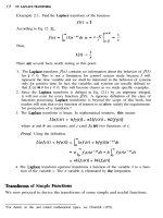
(i.e., x ≤ y =⇒ f(y) ≤ f(x)).
If the function f admits a continuous derivative f

, then the integration
formula
f(y)=f(x)+

y
x
f

(t) dt
leads to a sufficient condition for f to be decreasing: that f

(t) be nonposi-
tive for each t. It is easy to see that this is necessary as well, so a satisfying
characterization via f

is obtained.
If we go beyond the class of continuously differentiable functions, the sit-
uation becomes much more complex. It is known, for example, that there
exists a strictly decreasing continuous f for which we have f


(t) = 0 almost
everywhere. For such a function, the derivative appears to fail us, insofar
as characterizing decrease is concerned.
In 1878, Ulysse Dini introduced certain constructs, one of which is the
following (lower, right) derivate:
Df(x) := lim inf
t↓0
f(x + t) − f(x)
t
.
Note that Df(x)canequal+∞ or −∞.ItturnsoutthatDf will serve
our purpose, as we now see.
1 Analysis Without Linearization 3
1.1. Theorem. The continuous function f : R → R is decreasing iff
Df(x) ≤ 0 ∀x ∈ R.
Although this result is well known, and in any case greatly generalized in
a later chapter, let us indicate a nonstandard proof of it now, in order
to bring out two themes that are central to this book: optimization and
nonsmooth calculus.
Note first that Df(x) ≤ 0 is an evident necessary condition for f to be
decreasing, so it is the sufficiency of this property that we must prove.
Let x, y be any two numbers with x<y. We will prove that for any δ>0,
we have
min

f(t): y ≤ t ≤ y + δ

≤ f(x). (1)
This implies f(y) ≤ f(x), as required.

As a first step in the proof of (1), let g be a function defined on (x−δ, y +δ)
with the following properties:
(a) g is continuously differentiable, g(t) ≥ 0, g(t)=0ifft = y;
(b) g

(t) < 0fort ∈ (x − δ, y)andg

(t) ≥ 0fort ∈ [y, y + δ); and
(c) g(t) →∞as t ↓ x − δ, and also as t ↑ y + δ.
It is easy enough to give an explicit formula for such a function; we will
not do so.
Now consider the minimization over (x −δ, y + δ) of the function f + g;by
continuity and growth, the minimum is attained at a point z. A necessary
condition for a local minimum of a function is that its Dini derivate be
nonnegative there, as is easily seen. This gives
D(f + g)(z) ≥ 0.
Because g is smooth, we have the following fact (in nonsmooth calculus!):
D(f + g)(z)=Df(z)+g

(z).
Since Df(z) ≤ 0 by assumption, we derive g

(z) ≥ 0, which implies that
z lies in the interval [y, y + δ). We can now estimate the left side of (1) as
follows:
min

f(t): y ≤ t ≤ y + δ

≤ f(z)

≤ f(z)+g(z)(sinceg ≥ 0)
≤ f(x)+g(x)(since z minimizes f + g).
4 0. Introduction
We now observe that the entire argument to this point will hold if g is
replaced by εg, for any positive number ε (since εg continues to satisfy
the listed properties for g). This observation implies (1) and completes the
proof.
We remark that the proof of Theorem 1.1 will work just as well if f , instead
of being continuous, is assumed to be lower semicontinuous,whichisthe
underlying hypothesis made on the functions that appear in Chapter 1.
An evident corollary of Theorem 1.1 is that a continuous everywhere dif-
ferentiable function f is decreasing iff its derivative f

(x)isalwaysnonpos-
itive, since when f

(x) exists it coincides with Df(x). This could also be
proved directly from the Mean Value Theorem, which asserts that when f
is differentiable we have
f(y) − f(x)=f

(z)(y − x)
for some z between x and y.
Proximal Subgradients
We will now consider monotonicity for functions of several variables. When
x, y are points in R
n
, the inequality x ≤ y will be understood in the
component-wise sense: x
i

≤ y
i
for i =1, 2, ,n. We say that a given
function f : R
n
→ R is decreasing provided that f(y) ≤ f(x) whenever
x ≤ y.
Experience indicates that the best way to extend Dini’s derivates to func-
tions of several variables is as follows: for a given direction v in R
n
we
define
Df(x; v) := lim inf
t↓0
w→v
f(x + tw) − f(x)
t
.
We call Df(x; v)adirectional subderivate.LetR
n
+
denote the positive or-
thant in R
n
:
R
n
+
:= {x ∈ R
n

: x ≥ 0}.
We omit the proof of the following extension of Theorem 1.1, which can be
given along the lines of that of Theorem 1.1.
1.2. Theorem. The continuous function f : R
n
→ R is decreasing iff
Df(x; v) ≤ 0 ∀x in R
n
, ∀v ∈ R
n
+
.
When f is continuously differentiable, it is the case that Df(x; v) agrees
with

∇f(x),v

, an observation that leads to the following consequence of
the theorem:
1.3. Corollary. A continuously differentiable function f : R
n
→ R is de-
creasing iff ∇f(x) ≤ 0 ∀x ∈ R
n
.
1 Analysis Without Linearization 5
Since it is easier in principle to examine one gradient vector than an infinite
number of directional subderivates, we are led to seek an object that could
replace ∇f(x) in a result such as Corollary 1.3, when f is nondifferentiable.
A concept that turns out to be a powerful tool in characterizing a variety

of functional properties is that of the proximal subgradient. A vector ζ in
R
n
is said to be a proximal subgradient of f at x provided that there exist
a neighborhood U of x and a number σ>0 such that
f(y) ≥ f(x)+ζ,y − x−σy −x
2
∀y ∈ U.
The set of such ζ,ifany,isdenoted∂
P
f(x) and is referred to as the proximal
subdifferential. The existence of a proximal subgradient ζ at x corresponds
to the possibility of approximating f from below (thus in a one-sided man-
ner) by a function whose graph is a parabola. The point

x, f(x)

is a
contact point between the graph of f and the parabola, and ζ is the slope
of the parabola at that point. Compare this with the usual derivative, in
which the graph of f is approximated by an affine function.
Among the many properties of ∂
P
f developed later will be a Mean Value
Theorem asserting that for given points x and y, for any ε>0, we have
f(y) − f(x) ≤ζ,y −x + ε,
where ζ belongs to ∂
P
f(z) for some point z which lies within ε of the
line segment joining x and y. This theorem requires of f merely lower

semicontinuity. A consequence of this is the following.
1.4. Theorem. A lower semicontinuous function f : R
n
→ R is decreasing
iff ζ ≤ 0 ∀ζ in ∂
P
f(x), ∀x in R
n
.
We remark that Theorem 1.4 subsumes Theorem 1.2, as a consequence of
the following implication, which the reader may readily confirm:
ζ ∈ ∂
P
f(x)=⇒ Df(x; v) ≥ζ,v∀v.
While characterizations such as the one given by Theorem 1.4 are of in-
trinsic interest, it is reassuring to know that they can be and have been of
actual use in practice. For example, in developing an existence theory in
the calculus of variations, one approach leads to the following function f:
f(t):=max


1
0
L

s, x(s), ˙x(s)

ds: ˙x
2
≤ t


,
where the maximum is taken over a certain class of functions x:[0, 1] → R
n
,
and where the function L is given. In the presence of the constraint ˙x
2
≤
t, the maximum is attained, but the object is to show that the maximum is
6 0. Introduction
attained even in the absence of that constraint. The approach hinges upon
showing that for t sufficiently large, the function f becomes constant. Since
f is increasing by definition, this amounts to showing that f is (eventually)
decreasing, a task that is accomplished in part by Theorem 1.4, since there
is no a priori reason for f to be smooth.
This example illustrates how nonsmooth analysis can play a partial but
useful role as a tool in the analysis of apparently unrelated issues; detailed
examples will be given later in connection with control theory.
It is a fact that ∂
P
f(x) can in general be empty almost everywhere (a.e.),
even when f is a continuously differentiable function on the real line.
Nonetheless, as illustrated by Theorem 1.4, and as we will see in much
more complex settings, the proximal subdifferential determines the pres-
ence or otherwise of certain basic functional properties. As in the case of
the derivative, the utility of ∂
P
f is based upon the existence of a calculus
allowing us to obtain estimates (as in the proximal version of the Mean
Value Theorem cited above), or to express the subdifferentials of compli-

cated functionals in terms of the simpler components used to build them.
Proximal calculus (among other things) is developed in Chapters 1 and 3,
in a Hilbert space setting.
Generalized Gradients
We continue to explore the decrease properties of a given function f : R
n
→
R, but now we introduce, for the first time, an element of volition: we wish
to find a direction in which f decreases.
If f is smooth, linearization provides an answer: Provided that ∇f(x) =0,
the direction v := −∇f(x) will do, in the sense that
f(x + tv) <f(x)fort>0 sufficiently small. (2)
What if f is nondifferentiable? In that case, the proximal subdifferential
∂
P
f(x) may not be of any help, as when it is empty, for example.
If f is locally Lipschitz continuous, there is another nonsmooth calculus
available, that which is based upon the generalized gradient ∂f(x). A locally
Lipschitz function is differentiable almost everywhere; this is Rademacher’s
Theorem, which is proved in Chapter 3. Its derivative f

generates ∂f(x)
as follows (“co” means “convex hull”):
∂f(x)=co

lim
i→∞
∇f(x
i
): x

i
→ x, f

(x
i
) exists

.
Then we have the following result on decrease directions:
1.5. Theorem. The generalized gradient ∂f(x) is a nonempty compact
convex set. If 0 ∈ ∂f(x),andifζ is the element of ∂f(x) having minimal
norm, then v := −ζ satisfies (2).
2 Flow-Invariant Sets 7
The calculus of generalized gradients (Chapter 2) will be developed in an
arbitrary Banach space, in contrast to proximal calculus.
Lest our discussion of decrease become too monotonous, we turn now to
another topic, one which will allow us to preview certain geometric concepts
that lie at the heart of future developments. For we have learned, since
Dini’s time, that a better theory results if functions and sets are put on an
equal footing.
2 Flow-Invariant Sets
Let S be a given closed subset of R
n
and let ϕ: R
n
→ R
n
be locally
Lipschitz. The question that concerns us here is whether the trajectories
x(t) of the differential equation with initial condition

˙x(t)=ϕ

x(t)

,x(0) = x
0
, (1)
leave S invariant, in the sense that if x
0
lies in S,thenx(t) also belongs to S
for t>0. If this is the case, we say that the system (S, ϕ)isflow-invariant.
As in the previous section (but now for a set rather than a function),
linearization provides an answer when the set S lends itself to it; that is, it
is sufficiently smooth. Suppose that S is a smooth manifold, which means
that locally it admits a representation of the form
S =

x ∈ R
n
: h(x)=0

,
where h: R
n
→ R
m
is a continuously differentiable function with a nonva-
nishing derivative on S. Then if the trajectories of (1) remain in S,wehave
h


x(t)

=0fort ≥ 0. Differentiating this for t>0givesh


x(t)

˙x(t)=0.
Substituting ˙x(t)=ϕ

x(t)

, and letting t decrease to 0, leads to

∇h
i
(x
0
),ϕ(x
0
)

=0 (i =1, 2, ,m).
The tangent space to the manifold S at x
0
is by definition the set

v ∈ R
n
:


∇h
i
(x
0
),v

=0,i=1, 2, ,m

,
so we have proven the necessity part of the following:
2.1. Theorem. Let S be a smooth manifold. For (S, ϕ) to be flow-invariant,
it is necessary and sufficient that, for every x ∈ S, ϕ(x) belong to the tan-
gent space to S at x.
There are situations in which we are interested in the flow invariance of a set
which is not a smooth manifold, for example, S = R
n
+
, which corresponds
to x(t) ≥ 0.Itwillturnoutthatitisjustassimpletoprovethesufficiency
8 0. Introduction
part of the above theorem in a nonsmooth setting, once we have decided
upon how to define the notion of tangency when S is an arbitrary closed
set. To this end, consider the distance function d
S
associated with S:
d
S
(x):=min


x − s: s ∈ S

,
a globally Lipschitz, nondifferentiable function that turns out to be very
useful. Then, if x(·) is a solution of (1), where x
0
∈ S,wehavef(0) = 0,
f(t) ≥ 0fort ≥ 0, where f is the function defined by
f(t):=d
S

x(t)

.
What property would ensure that f(t)=0fort ≥ 0; that is, that x(t) ∈ S?
Clearly, that f be decreasing: monotonicity comes again to the fore! In the
light of Theorem 1.1, f is decreasing iff Df(t) ≤ 0, a condition which at
t =0says
lim inf
t↓0
d
S
(x(t))
t
≤ 0.
Since d
S
is Lipschitz, and since we have
x(t)=x
0

+ tϕ(x
0
)+o(t),
the lower limit in question is equal to
lim inf
t↓0
d
S
(x
0
+ tϕ(x
0
))
t
.
This observation suggests the following definition and essentially proves the
ensuing theorem, which extends Theorem 2.1 to arbitrary closed sets.
2.2. Definition. A vector v is tangent to a closed set S at a point x if
lim inf
t↓0
d
S
(x + tv)
t
=0.
The set of such vectors is a cone, and is referred to as the Bouligand tangent
cone to S at x, denoted T
B
S
(x). It coincides with the tangent space when

S is a smooth manifold.
2.3. Theorem. Let S be a closed set. Then (S, ϕ) is flow-invariant iff
ϕ(x) ∈ T
B
S
(x) ∀x ∈ S.
When S is a smooth manifold, its normal space at x is defined as the space
orthogonal to its tangent space, namely
span

∇h
i
(x): i =1, 2, ,m

,
2 Flow-Invariant Sets 9
and a restatement of Theorem 2.1 in terms of normality goes as follows:
(S, ϕ) is flow-invariant iff

ζ,ϕ(x)

≤ 0 whenever x ∈ S and ζ is a normal
vector to S at x.
We now consider how to develop in the nonsmooth setting the concept
of an outward normal to an arbitrary closed subset S of R
n
.Thekeyis
projection:Givenapointu not in S, and let x be a point in S that is closest
to u;wesaythatx lies in the projection of u onto S. Then the vector u −x
(and all its nonnegative multiples) defines a proximal normal direction to

S at x. The set of all vectors constructed this way (for fixed x,byvarying
u) is called the proximal normal cone to S at x, and denoted N
P
S
(x). It
coincides with the normal space when S is a smooth manifold.
It is possible to characterize flow-invariance in terms of proximal normals
as follows:
2.4. Theorem. Let S be a closed set. Then (S, ϕ) is flow-invariant iff

ζ,ϕ(x)

≤ 0 ∀ζ ∈ N
P
S
(x), ∀x ∈ S.
We can observe a certain duality between Theorems 2.3 and 2.4. The former
characterizes flow-invariance in terms internal to the set S, via tangency,
while the latter speaks of normals generated by looking outside the set.
In the case of a smooth manifold, the duality is exact: the tangential and
normal conditions are restatements of one another. In the general non-
smooth case, this is no longer true (pointwise, the sets T
B
S
and N
P
S
are not
obtainable one from the other).
While the word “duality” may have to be interpreted somewhat loosely,

this element is an important one in our overall approach to developing non-
smooth analysis. The dual objects often work well in tandem. For example,
while tangents are often convenient to verify flow-invariance, proximal nor-
mals lie at the heart of the “proximal aiming method” used in Chapter 4
to define stabilizing feedbacks.
Another type of duality that we seek involves coherence between the various
analytical and geometrical constructs that we define. To illustrate this,
consider yet another approach to studying the flow-invariance of (S, ϕ), that
which seeks to characterize the property (cited above) that the function
f(t)=d
S

x(t)

be decreasing in terms of the proximal subdifferential of f
(rather than subderivates). If an appropriate “chain rule” is available, then
we could hope to use it in conjunction with Theorem 1.4 in order to reduce
the question to an inequality:

∂
P
d
S
(x),ϕ(x)

≤ 0 ∀x ∈ S.
Modulo some technicalities that will interest us later, this is feasible. In the
light of Theorem 2.4, we are led to suspect (or hope for) the following fact:
N
P

S
(x) = the cone generated by ∂
P
d
S
(x).
10 0. Introduction
This type of formula illustrates what we mean by coherence between con-
structs, in this case between the proximal normal cone to a set and the
proximal subdifferential of its distance function.
3 Optimization
As a first illustration of how nonsmoothness arises in the subject of opti-
mization, we consider minimax problems. Let a smooth function f depend
on two variables x and u, where the first is thought of as being a choice
variable, while the second cannot be specified; it is known only that u varies
in a set M. We seek to minimize f .
Corresponding to a choice of x, the worst possibility over the values of u
that may occur corresponds to the following value of f :max
u∈M
f(x, u).
Accordingly, we consider the problem
minimize
x
g(x), where g(x):=max
u∈M
f(x, u).
The function g so defined will not generally be smooth, even if f is a nice
function and the maximum defining g is attained. To see this in a simple
setting, consider the upper envelope g of two smooth functions f
1

, f
2
.(We
suggest that the reader make a sketch at this point.) Then g will have a
corner at a point x where f
1
(x)=f
2
(x), provided that
f

1
(x) = f

2
(x).
Returning to the general case, we remark that under mild hypotheses, the
generalized gradient ∂g(x) can be calculated; we find
∂g(x)=co

f

x
(x, u): u ∈ M(x)

,
where
M(x):=

u ∈ M : f(x, u)=g(x)


.
This characterization can then serve as the initial step in approaching the
problem, either analytically or numerically. There may then be explicit
constraints on x to consider.
A problem having a very specific structure, and one which is of considerable
importance in engineering and optimal design, is the following eigenvalue
problem. Let the n × n symmetric matrix A depend on a parameter x
in some way, so that we write A(x). A familiar criterion in designing the
underlying system which is represented by A(x) is that the maximal eigen-
valueΛofA(x) be made as small as possible. This could correspond to a
question of stability, for example.
3 Optimization 11
It turns out that this problem is of minimax type, for by Rayleigh’s formula
for the maximal eigenvalue we have
Λ(x)=max

u, A(x)u: u =1

.
The function Λ(·) will generally be nonsmooth, even if the dependence
x → A(x) is itself smooth. For example, the reader may verify that the
maximal eigenvalue Λ(x, y) of the matrix
A(x, y):=

1+xy
y 1 − x

is given by 1 +



(x, y)


. Note that the minimum of this function occurs at
(0, 0), precisely its point of nondifferentiability. This is not a coincidence,
and it is now understood that nondifferentiability is to be expected as
an intrinsic feature of design problems generally, in problems as varied as
designing an optimal control or finding the shape of the strongest column.
Another class of problems in which nondifferentiability plays a role is that of
L
1
-optimization. In its discrete version, the problem consists of minimizing
a function f of the form
f(x):=
p

i=1
m
i
x − s
i
. (1)
Such problems arise, for example, in approximation and statistics, where
L
1
-approximation possesses certain features that can make it preferable to
the more familiar (and smooth) L
2
-approximation.

Let us examine such a problem in the context of a simple physical system.
Torricelli’s Table
A table has holes in it at points whose coordinates are s
1
, s
2
, ,s
p
.Strings
are attached to masses m
1
, m
2
, ,m
p
, passed through the corresponding
hole, and then are all tied to a point mass m whose position is denoted
x (see Figure 0.1). If friction and the weight of the strings are negligible,
the equilibrium position x of the nexus is precisely the one that minimizes
the function f given by (1), since f (x) can be recognized as the potential
energy of the system.
The proximal subdifferential of the function x →x −s is the closed unit
ball if x = s, and otherwise is the singleton set consisting of its derivative,
the point (x − s)

x −s. Using this fact, and some further calculus, we
can derive the following necessary condition for a point x to minimize f;
0 ∈
p


i=1
m
i
∂
P
(·) − s
i
(x). (2)
12 0. Introduction
FIGURE 0.1. Torricelli’s table.
Of course, (2) is simply Fermat’s rule in subdifferential terms, interpreted
for the particular function f that we are dealing with.
There is not necessarily a unique point x that satisfies relation (2), but
it is the case that any point satisfying (2) globally minimizes f .Thisis
because f is convex, another functional class that plays an important role
in the subject. A consequence of convexity is that there are no purely local
minima in this problem.
When p = 3, each m
i
= 1, and the three points are the vertices of a
triangle, the problem becomes that of finding a point such that the sum
of its distances from the vertices is minimal. The solution is called the
Torricelli point, after the seventeenth-century mathematician.
The fact that (2) is necessary and sufficient for a minimum allows us to
recover easily certain classical conclusions regarding this problem. As an
example, the reader is invited to establish that the Torricelli point coincides
with a vertex of the triangle iff the angle at that vertex is 120
◦
or more.
Returning now to the general case of our table, it is possible to make

the system far more complex by the addition of one more string and one
more mass m
0
,ifweallowthatmasstohangovertheoutsideedgeofthe
table. Then the extra string will automatically trace a line segment from
x toapoints(x) on the edge of the table that is closest to x (locally at
least, in the sense that s(x) is the closest point to x on the edge, relative
to a neighborhood of s(x).) If S is the set defined as the closure of the
complement of the table, the potential energy (up to a constant) of the