ECOTOXICOLOGY: A Comprehensive Treatment - Chapter 8 potx

Clements: “3357_c008” — 2007/11/9 — 18:10 — page 115 — #1
8
Models of
Bioaccumulation
and Bioavailability
8.1 OVERVIEW
The object of this work will consist in the derivation of general mathematical relations from which it is
possible, at least for practical purposes, to describe the kinetics of distribution of substances in the body.
(Teorell 1937a)
There are well-established ways to quantify bioaccumulation. Some mathematical models give parsi-
monious description or restricted prediction for a particular exposure scenario. As reflected in the
above quote from Teorell’s classic paper in which these methods were first introduced, such models
are focused on practicality. More complicated models describe or predict bioaccumulation in a more
general way based on physiological, biochemical, and anatomical features. Most simple models
employ mathematical compartments while complicated models describe exchange among several
interconnected physical or biochemical compartments. Many combine features of both modeling
extremes.Although initially appearing as ajumble of competing approaches, this blend of approaches
makes sense in ecotoxicology: some scenarios require a simple, pragmatic model but more involved
models might be needed to capture the essential features of the situation under study. This is con-
sistent with the general tenet that a model should be no more complicated than needed to answer the
question being asked. For cases in which accurate description or prediction is paramount for many
diverse species, contaminants, or conditions, a more complicated model incorporating physiolo-
gical, biochemical, and anatomical features likely will be the best alternative. Otherwise, many
simple models each of which only describes one relevant species/toxicant/condition combination
would have to be employed.
Similarly, estimations of contaminant bioavailability from relevant sources can be produced for a
particular situation using simple empirical models or more generally by applying predictive models
based on in-depth mechanistic knowledge. Like bioaccumulation models, which bioavailability
approach is the most appropriate depends on the study goals and the desired generality of the results.
8.2 BIOACCUMULATION
Most bioaccumulation models translate an external concentration to an internal concentration that is

then related to an effect. The form of the model depends on the media containing the contaminant,
qualities of the environment in which the exposuretakes place, and the qualities ofthe organism itself.
Models for nonionic organic compound uptake via gills might incorporate general equations based
on lipid solubility relationships. Models for weakly acidic or basic compounds ingested in food might
incorporate pH Partition Theory using the Henderson–Hasselbalch equations. Models for dissolved
metal uptake across gill surfaces might be formulated using free ion activity model (FIAM) or biotic
ligand model (BLM) based relationships. For example, a FIAM relationship might be developed for
a dissolved metal being taken up under different pH, temperature, or water quality conditions that
115
© 2008 by Taylor & Francis Group, LLC
Clements: “3357_c008” — 2007/11/9 — 18:10 — page 116 — #2
116 Ecotoxicology: A Comprehensive Treatment
influence chemical speciation. Allometric
1
power equations might be incorporated if the organism
grows substantially during the period of bioaccumulation. Still other models need to accommodate
the interactions between physical and biological qualities. For example, temperature’s influence on
chlorpyrifos uptake is different for insect groups differing in respiratory strategy (Buchwalter et al.
2003). There are basic similarities among most models although a model might take slightly different
forms depending on the exposure scenario and objectives of the modeling effort. These fundamental
similarities will be highlighted in the next few pages.
8.2.1 UNDERLYING MECHANISMS
The exact formulation of a bioaccumulation model depends on the underlying mechanisms of uptake,
internal redistribution, and elimination. As detailed in Chapter 7, some compounds are taken up or
eliminated by mechanisms that can be saturated or modified by competition with other compounds.
Bioaccumulation of others is influenced by factors such as urine or gut pH, and inclusion of these
factors in the associated model might berequired. Still other processes can be modifiedbyacclimation
or damage. Some compounds are subject to internal breakdown but others are not.
8.2.2 ASSUMPTIONS OF MODELS AND METHODS OF FITTING DATA
Models are developed based on three different formulations: rate-constant-based, clearance-volume-

based, and fugacity-based formulations. All are equivalent in their basic forms, but each formulation has
its own advantages and disadvantages.
(Newman and Unger 2003)
Models are based on mathematical expediency (descriptive models), processes and structures
described in earlier chapters (mechanistic models), or a blending of both. The most common assump-
tions revolve around reaction order for the relevant processes so it is worth taking a moment to review
the fundamentals of zero, first, and mixed order reactions. Recollect that order for a reaction or pro-
cess involving one reactant refers to the power to which concentration is raised in the differential
equation describing the associated kinetics, for example,
Zero order:
dC
dt
=−kC
0
=−k,
First order:
dC
dt
=−kC
1
=−kC.
The equations above are expressed for elimination so the change in internal concentration is
denoted by −k or −kC: concentrations are decreasing with time. For uptake, the sign would be
positive. The generic k denoted here is a simple proportionality or rate constant. Continuing the
example with elimination, a plot of concentration (C
t
) versus time (t) will produce a straight line
for zero order processes: the absolute value of the slope of that line is an estimate of k. The zero
order k has units of C/t. For first order processes, ln C
t

is plotted against t to produce a straight line
and the absolute value of the slope is k. Alternatively, one could plot the ln(C
t
/C
t=0
) against time
for processes following first order kinetics. The slope would then be k (Piszkiewicz 1977). The units
for the first order k are 1/t; however, we will see that some slightly more involved bioaccumulation
models apply a “first order k” for some processes that have different units.
Saturation kinetics used to describe carrier-mediated membrane transport or enzyme-mediated
breakdown of a compound are slightly more complicated. Let S be the compound being acted on, by
1
Allometry is the study of organism size and its consequences.
© 2008 by Taylor & Francis Group, LLC
Clements: “3357_c008” — 2007/11/9 — 18:10 — page 117 — #3
Models of Bioaccumulation and Bioavailability 117
either enzymatic conversion or transport by a carrier molecule, E be the enzyme or carrier molecule,
and P be the product of enzyme conversion or the compound successfully transported across the
membrane via the carrier:
S + E
k
−1

k
+1
ES
k
−2

k

+2
E +P.
The differential equation describing the change in substrate through time would be
dC
S
dt
=−k
+1
C
E
C
S
+k
−1
C
ES
, (8.1)
where C
S
, C
E
, and C
ES
are the concentrations of S, E, and ES, respectively. If one were to plot the
curve of C
S
versus time, the apparent order would depend on the initial C
S
and might change as
C

S
changes through time. Above a certain C
S
, the enzyme or membrane transport system would
be saturated and incapable of converting/transporting S any faster than a characteristic maximum
velocity (V
max
): the C
S
versus time curve would appear to conform to zero order kinetics above the
saturation concentration. If one started with very low C
S
relative to the saturation concentration,
the curve would appear to describe first order kinetics. The Michaelis–Menten equation predicting
the rate (v) at which conversion occurs for such a process is the following:
v =
V
max
C
S
k
m
+C
S
, (8.2)
where k
m
is the C
S
at which v is half of V

max
. Like concentration–time curves for zero and first
order processes, there are several ways to estimate parameters for saturation kinetics, including the
most commonly applied double-reciprocal (Lineweaver–Burk) plot and three less common plots
(Eadie–Hofstee, Scatchard, and Woolf plots). Traditionally, a series of C
S
are established in mixture
with the same concentration of enzyme and the rate of disappearance of S (or appearance of P) is
measured for each concentration. The C
S
and conversion rates (v) are then plotted or fit by linear
regression to estimate V
max
and k
s
. Raaijmaker (1987) discusses the statistical concerns associated
with these transformations, concluding that the Woolf plot functions best.
Lineweaver–Burk:
1
v
=
k
m
+C
S
V
max
C
S
=

1
V
max
+
k
m
V
max
C
S
, (8.3)
Eadie–Hofstee: v = V
max
−
k
m
v
C
S
, (8.4)
Scatchard:
v
C
S
=
V
max
k
m
−

v
k
m
, (8.5)
Woolf :
C
S
v
=
k
m
V
max
+
C
S
V
max
. (8.6)
Piszkiewicz (1977) provides details for deriving these transformations and relating one to the
other.
Of course, a nonlinear model can also be fit directly to the v versus C
S
data to parameterize the
Michaelis–Menten model. If such fitting involves an iterative maximum likelihood approach, the
estimates from one of the above linearizing plots might be used as initial values. It might be more
convenient during some modeling efforts to assume zero order kinetics above a certain concentration
and then first order when concentrations drop below saturation during a time course. Because the time
it will take for the concentration to fall below saturation depends on the initial concentration, it would
© 2008 by Taylor & Francis Group, LLC

Clements: “3357_c008” — 2007/11/9 — 18:10 — page 118 — #4
118 Ecotoxicology: A Comprehensive Treatment
be convenient to be able to estimate when one should shift from zero to first order computations.
Wagner (1979) provides a convenient relationship for estimating the time to transition from zero to
first order (t
∗
) as a function of the initial concentration (C
S0
):
t
∗
=

1 − (1/e)
V
max

C
S0
+
k
m
V
max
. (8.7)
Box 8.1 Silver Transport across Membranes Exhibits Saturation Kinetics
Because the silver ion, Ag
+
, is highly toxic to freshwater fishes, its transport across and effects
on gills is a very active area of research. As one example, Bury et al. (1999) characterized

silver transport by a Na
+
/K
+
-ATPase located on the basolateral membranes of gill cells using
a conventional saturation kinetics model. This study is ideal for illustrating here the relevance
of saturation kinetics for one feature of contaminant bioaccumulation.
Bury et al. (1999) describe studies published preceding theirs in which the Ag
+
ion was
shown to be transported into gill cells by a Na
+
channel subject to saturation kinetics. Because
P-type ATPases
2
had been documented for other metals, Bury et al. hypothesized that Ag
+
might also be transported by ATPases in rainbow trout (Oncorhynchus mykiss) gill membrane
vesicles. They removed gills from trout and produced membrane vesicles by a sequence of
homogenization, agitation, and centrifugation steps. Radioactive silver (
110m
Ag) was then used
to measure movement of Ag
+
into isolated gill cell membrane vesicles.
Supporting the hypothesis of Bury and coworkers, the Ag
+
transport into the vesicles
was found to be ATP dependent. Competitive inhibition was also apparent from experiments
showing that Ag

+
transport slowed if Na
+
or K
+
concentrations were increased in the media
surrounding the vesicles. Michaelis–Menten parameters were estimated by fitting the nonlinear
Michaelis–Menten model (Equation 8.2) to vesicle uptake (nmolofAg
+
/mg protein/min) versus
Ag concentration (µmol). The V
max
was 14.3 nmol/mg membrane protein/min and the K
m
was
62.6 µmol. An Eadie–Hofstee plot produced straight lines and also was used to fit these data
by linear regression methods. Bury et al. concluded that there was a P-type ATPase transport
mechanism for silver in trout gills and defined the characteristics of the saturation kinetics in
vesicle preparations.
8.2.3 RATE CONSTANT-BASED MODELS
[The assumption of a single compartment] may not be applied to all drugs. For most drugs, concentrations
in plasma measured shortly after iv injection reveal a distinct distributive phase. This means that a
measurable fraction of the dose is eliminated before attainment of distribution equilibrium. These drugs
impart the characteristics of a multicompartment system upon the body. No more than two compartments
are usually needed to describe the time course of drug in the plasma. These are often called the rapidly
equilibrating or central compartment and the slowly equilibrating or peripheral compartment.
(Gibaldi 1991)
Without a doubt, the most commonly applied bioaccumulation model in ecotoxicology is a
one-compartment model with onefirst order uptake and one first order elimination term.After gaining
entry, the toxicant is assumed to instantly distribute itself uniformly within that compartment. There

2
P-typeATPases are one of three categories ofATPases. They are ubiquitous in living systems, facilitating cation transport
for a variety of functions. The formation of a phosphorylated intermediate during transport leads to their designation as P-type.
© 2008 by Taylor & Francis Group, LLC
Clements: “3357_c008” — 2007/11/9 — 18:10 — page 119 — #5
Models of Bioaccumulation and Bioavailability 119
is no hysteresis, that is, the likelihood of a molecule of the toxicant leaving the compartment is
independent of how long it has been in the compartment. The relevant model can be constructed
easily with the information covered already. The elimination from the compartment would simply
be the following:
dC
i
dt
=−k
e
C
i
, (8.8)
where C
i
is the internal concentration (or amount) of the compartment and k
e
is the first order rate
constant (1/t). As already discussed, the k
e
for such elimination can be estimated by fitting a linear
regression line to ln C
i
at different times (ln C
i,t

) versus time (t). The antilog of the y-intercept of
the regression line can also be used to estimate the initial concentration in the compartment, C
i,0
.
Because this estimate can be biased, Newman (1995) provides a method of removing any bias
from an estimated C
i,0
. This differential equation (8.8) can be integrated to predict the concentration
remaining in the compartment through time, perhapsafterasource has been removed
3
or the organism
has been dosed once and then allowed to eliminate the toxicant:
C
i,t
= C
i,0
e
−k
e
t
. (8.9)
Useful metrics associated with this simple elimination model include the biological half-life of
the toxicant in the compartment (t
1/2
) (Equation 8.10) and the mean residence (or turnover) time of
a toxicant molecule in the compartment (τ ) (Equation 8.11):
t
1/2
=
ln 2

k
e
(8.10)
τ =
1
k
e
. (8.11)
Equation 8.12 can be used to model elimination if there are two components of elimination that
remove the toxicant from one compartment:
C
i,t
= C
i,0
e
−(k
e,1
+k
e,2
)t
. (8.12)
If a compartment were composed of two subcompartments with no exchange between them, the
change in the total concentration or amount in the two combined subcompartments (1 and 2) could
be estimated by
C
i,t
= C
0,1
e
−k

e,1
t
+C
0,2
e
−k
e,2
t
. (8.13)
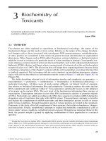
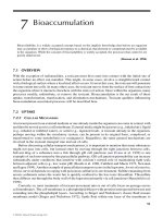
Figure 8.1 depicts the change in total concentration (or amount) in such a situation. In that figure,
the two subcompartments are designated “fast” and “slow.” A plot of ln C for the compartment that
appears to be composed of the two subcompartments versus time of elimination will result in a curve
composed of two linear segments. The linear segment for the laterportion of the total curve will reflect
the change in concentration (or amount) in the slow subcompartment because the compound in the fast
compartment will have been eliminated by that time in the course of depuration. The linear segment
at the beginning of the depuration period will reflect the combined concentration in both the slow and
fast subcompartments. The two elimination components can be modeled by nonlinear regression or a
3
An experimental design or action in which an organism containing a toxicant is removed to a clean environment where
it can eliminate the toxicant is called a depuration design. The elimination of toxicant after movement to a clean environment
is called depuration.
© 2008 by Taylor & Francis Group, LLC
Clements: “3357_c008” — 2007/11/9 — 18:10 — page 120 — #6
120 Ecotoxicology: A Comprehensive Treatment
Time
ln concentration
Predominantly slow eliminatio
n component
Mixture of fast and slow
elimination components

Backstripped fast component
ln C
0
,
Slow
ln C
0
,
Fast
FIGURE 8.1 The elimination of compound from a compartment composed of two subcompartments with
no exchange of compound between compartments. Both subcompartments have one, first order elimination
component.
conventional backstripping method. To begin the backstripping approach, a line is fit to the portion of
the curve that is predominantly associated with “slow” elimination. The y-intercept of the regression
line is the ln C
0,Slow
and the absolute value of the slope is the k
e,Slow
. The C
0,Fast
and k
e,Fast
are
then estimated using the data for the line segment associated with the combined concentrations in
the two compartments through time and the regression model. The regression model for the slow
component is used to predict how much of the concentration of compound measured during the
initial linear phase of depuration was associated with the slow component. These predictions are
subtracted from the observed concentrations to estimate the amount associated only with the fast
elimination component. In essence, the concentration associated with the slow component is stripped
away, leaving only that associated with the fast component. These “fast elimination” predictions for

each data point would be distributed about the “backstripped” line depicted in Figure 8.1. A linear
regression model is fit to these predictions, and the y-intercept and slope used as just described for
the slow elimination component to predict C
0,Fast
and k
e,Fast
. This same general procedure can also
be used if more than two components are present.
The uptake from an external source with a constant concentration (C
x
) can be defined as the
following:
dC
i
dt
= k
u
C
x
, (8.14)
where k
u
is the first order rate constant for uptake (1/t). As we will see, the units of k
u
will change
when Equations 8.8 and 8.14 are combined and applied to model bioaccumulation in many cases.
Combining these two equations, bioaccumulation for a single compartment model can be described
with the following:
dC
i

dt
= k
u
C
x
−k
e
C
i
. (8.15)
The above equation can be integrated to yield the conventional single compartment model with
one uptake and one elimination term, both of which conform to first order kinetics:
C
i,t
= C
x
k
u
k
e
[1 − e
−k
e
t
]. (8.16)
© 2008 by Taylor & Francis Group, LLC
Clements: “3357_c008” — 2007/11/9 — 18:10 — page 121 — #7
Models of Bioaccumulation and Bioavailability 121
A simple adjustment to Equation 8.16 provides some insight about conditions as concentrations
inside the organism approach steady state conditions with the external source. As t gets very large,

the bracketed term in Equation 8.16 approaches 1; the bracketed term falls out of the equation
as concentrations approach steady state. If both sides of the equation are then divided by C
S
,it
becomes apparent that the quotient of the concentration in the organism at steady state and external
concentration (C
∞
/C
x
) is equal to k
u
/k
e
. If this model described uptake from water, the k
u
/k
e
would
then be an estimate of the bioconcentration factor (BCF).
It is important to note that the constants are conditional if this model described the kinetics for
compartments of differentsizes. The size ofthebiologicalcompartmentandthatoftheexternalsource
compartment influence the k
u
value. If two individuals of identical volume were placed into sources
of different volumes but identical concentrations, the estimated values of k
u
would be different
for each. Similarly, the k
u
values would be different for two different sized individuals exposed to

the same concentration of contaminant contained in the same volume of media. In reality, the k
u
is
the flux or clearance rate of the source by an individual of a specific size; therefore, the units of k
u
are
flow/mass, for example, (mL/h)/g, for the equation to balance properly. (SeeAppendix 5 in Newman
and Unger (2003) for a detailed dimensional analysis.) We will return to this important point of
considering compartment volumes after a brief elaboration on single-compartment bioaccumulation
models.
The rudimentary model defined by Equation 8.15 or 8.16 can be changed to meet the needs
of the modeler. Equation 8.16 can accommodate the confounding factor of the organism rep-
resented by the compartment having an initial concentration (C
0
) before the exposure being
modeled
C
i,t
= C
x
k
u
k
e
[1 − e
−k
e
t
]+C
i,0

e
−k
e
t
. (8.17)
Two elimination (Equation 8.18) or uptake (Equation 8.19 for uptake from water and food) terms
can be included in the model also:
C
i,t
= C
x
k
u
k
e1
+k
e2
[1 − e
−(k
e1
+k
e2
)t
], (8.18)
where k
e1
and k
e2
are the elimination rate constants for processes 1 and 2:
C

i,t
=
C
w
k
uw
+αRC
f
k
e
[1 − e
−k
e
t
], (8.19)
where C
w
and C
f
are concentrations in water and food, respectively, α is amount of compound
absorbed per amount of compound ingested, and R = the weight-specific ration. Obviously, the
exact form of any model will change to the most convenient one as sources change but the general
framework remains the same.
Returning to our discussion of volumes, compartment volumes also become relevant if the
organism was modeled as having two or more compartments that exchange compound. But how
are these volumes measured? As a simple illustration, a dose of the compound (D) is applied in
a one-compartment model and allowed enough time to evenly distribute in the compartment. The
compartment is sampled to determine the concentration (C), and then the compartment volume (V)
is estimated as D/C = V. The estimation of volumes becomes complicated if more than one
compartment is involved. How volumes are handled in such a situation can be illustrated with the

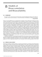
conventional, two-compartment models used often in pharmacology and ecotoxicology (Figure 8.2).
With such multiple compartments, volumes are expressed as apparent or effective volumes of dis-
tribution (V
d
) and treated as mathematically defined compartments that might or might not be easily
related to a physical compartment. The most common situation in which such volumes are employed
© 2008 by Taylor & Francis Group, LLC
Clements: “3357_c008” — 2007/11/9 — 18:10 — page 122 — #8
122 Ecotoxicology: A Comprehensive Treatment
Time
ln concentration
C
t
=C
A
e
−k
A
t
+ C
B
e
−k
B
t
D
A
B
k
BA

k
AB
k
A0
FIGURE 8.2 The estimation of compartment volumes for an organism modeled as two compartments with
exchange between compartments and a single dose, D. First order microconstants are also derived from the
macroconstants for concentration–time curve of the reference compartment (C
0,A
, C
0,B
, k
A
, k
B
). In many
cases, the reference compartment (A) is the blood (or plasma) and the peripheral compartment includes the
tissues with which the compound exchanges with the blood. More complex models are often warranted and
require more detailed computations.
would be one in which a compound is introduced into the blood and the concentrations are then fol-
lowed through time in the blood. The compound in the blood is envisioned as exchanging with some
other compartment. The V
d
for the nonblood (peripheral) compartment is expressedinunitsofvolume
of the blood (reference) compartment. For the two-compartment model depicted in Figure 8.2, the
microconstants and volumes of distribution for the compartments can be estimated with the following
relationships:
k
AB
=
C

A
k
B
+C
B
k
A
C
A
+C
B
(8.20)
k
A0
=
k
A
k
B
k
AB
(8.21)
k
AB
= k
A
+k
B
−k
AB

−k
A0
(8.22)
V
dA
=
D
C
A
+C
B
(8.23)
V
dB
= V
dA

k
AB
k
BA

. (8.24)
The steady-state V
d
for the entire organism consisting of the two compartments is the sum of
V
dA
and V
dB

. It is important to note that the steady state V
d
reflects the amount of compound in a
unit volume of the organism expressed in terms of the equivalent volume of the reference (source)
compartment that would contain that same amount of compound. So, the volume of the peripheral
compartment is expressed in units of the reference (blood) compartment. This holds true also if the
source (reference) compartment was the water surrounding the organism; the steady-state V
d
for the
organism compartment would be a measure of the BCF because it expresses the volume of organism
compartment that holds an equivalent amount of the chemical as a unit volume of the water source
compartment.
8.2.4 CLEARANCE VOLUME-BASED MODELS
Often, especially in the fields of pharmaco-or toxicokinetics, bioaccumulation models are formulated
in the context of clearance. Clearance is the volume of a compartment that is cleared of a substance
per unit time. In these kinds of models, one compartment, such as the blood or plasma, is selected as
© 2008 by Taylor & Francis Group, LLC
Clements: “3357_c008” — 2007/11/9 — 18:10 — page 123 — #9
Models of Bioaccumulation and Bioavailability 123
the reference compartment and clearances are calculated relative to that compartment. Clearances
can be expressed as volume/time or as mass-normalized clearances [(volume/time)/mass]. A quick
glance back to our previous discussions of k
u
in bioaccumulation models will show that the k
u
was
actually a clearance. Clearances (Cl) can be calculated for simple bioaccumulation models from
terms already discussed above (i.e., Cl = k
e
V

d
). By substitution, the rate constant-based model
shown in Equation 8.16 can be converted to a clearance-based model:
C
i,t
= C
x
V
d
[1 − e
−(Cl/V
d
)t
]. (8.25)
Following the reasoning used already for V
d
at steady state, it is easy to see again from Equation 8.25
that V
d
at steady state is equal to the quotient of the steady-state concentration in the organism
(compartment) to the source.
8.2.5 FUGACITY-BASED MODELS
Bioaccumulation models sometimes are formulated in terms of fugacity, the escaping tendency for
a substance from a medium or phase. Formulations using fugacity have the distinct advantage that
states and rates for all components in complex models can be expressed in the same units. This makes
mass balance equations much more tractable than with other approaches (Mackay 1979). Fugacity (f )
is expressed as a pressure (e.g., units of Pascal or Pa) and is derived from concentrations (C in units
of mol/m
3
), i.e., f = Z/C where Z is the fugacity capacity of the phase [mol/(m

3
Pa)]. The fugacity
capacity is “a kind of solubility or capacity of a phase to absorb the chemical” (Mackay 1979) so a
modeled compound tends to accumulate in phases or compartments with high fugacity capacities.
Because of this direct relationship between f and C, the steady state quotient of the concentration
in one phase or compartment to that in another (e.g., the BCF) is also equal to the quotient of the
fugacity capacities of the two compartments.
Only one definition and two identities are needed to convert the simple bioaccumulation models
shown in Equation 8.16 to a fugacity-based model. In fugacity-based models, the movement of a
substance between compartments is expressed as a transport rate (N, mol/h) and is calculated with a
transport constant (D, mol/h×Pa) and the difference in fugacities for the two compartments (f
1
−f
2
):
N = D[f
1
−f
2
]. (8.26)
The rate constant, D, can be used for a diverse range of relevant processes including chemical
reactions, diffusion, or advection (Mackay 2004), making it a very convenient term in complex envir-
onmental models. The conversion of k
u
and k
e
to terms used in fugacity modeling is straightforward
(Gobas and Mackay 1987):
k
e

=
D
0
V
0
Z
0
, (8.27)
k
u
= D
0
V
0
Z
S
, (8.28)
where D
0
= transport constant for the organism being modeled, V
0
= the volume of the organism
being modeled, Z
0
= a proportionality constant called the fugacity capacity for the organism, and
Z
S
= the fugacity capacity for the source of the substance being accumulated. With these definitions,
a simple fugacity-based model can be produced.
C

0,t
= C
x
Z
0
Z
S
[1 − e
−[D
0
/(V
0
Z
0
)]t
] (8.29)
© 2008 by Taylor & Francis Group, LLC
Clements: “3357_c008” — 2007/11/9 — 18:10 — page 124 — #10
124 Ecotoxicology: A Comprehensive Treatment
This model can be expressed in terms of fugacities instead of concentrations also (Gobas and
Mackay 1987):
f
0
= f
S
[1 − e
−[D
0
/(V
0

Z
0
)]t
]. (8.30)
Box 8.2 Unit and Real World Renderings with Fugacity Models
Fugacity simplifies and clarifies the relationship between equilibrium concentrations in various
fluids and solids. Rather than relate two concentrations using a partition coefficient , each
concentration is independently related to fugacity, and the two fugacities equated.
(Mackay 2004)
It seemed to me that by reformulating equations in terms of fugacity, environmental mass balances
could be done more easily, especially for systems involving disparate phases
(Mackay 2004)
With a toolbox containing f , Z, and D, the modeler has the key tools to quantify chemical fate in a
vast variety of situations from transport across a cell membrane to estimating global distribution of
chemical of commerce.
(Mackay 2004)
A brief look at the remarkable work of Don Mackay and his colleagues seems an appropriate
way to illustrate the value and universal applicability of fugacity-based contaminant modeling.
Fugacity-based models have been so influential that an entire issue of the journal Environmental
Toxicology and Chemistry (vol. 23, no. 10) was recently dedicated to them. Beyond MacKay’s
first paper introducing the fugacity concept for contaminant modeling (Mackay 1979), particu-
larly useful or exemplary publications applying this approach include Cahill et al. (2003), Czub
and McLachlan (2004), Gobas and Mackay (1987), Hickie et al. (1999), Mackay (1979, 2001),
Mackay and Wania (1995), and Wania and Mackay (1995). As described above in Mackay’s
own words, the great advantage of the fugacity approach is the ability to simplify models by
simplifying units. Equations for different processes such as diffusion, advection, or chemical
reaction could be made more consistent in this manner.
Mackay also facilitated environmental modeling by developing a series of fugacity-based
models of increasing complexity. These conceptual microcosms or “unit worlds” provided the
starting point for addressing numerous real-world questions. The simpler unit worlds included

a few compartments such as air, sediment, soil, and water. Among the more complicated unit
worlds is a Level III fugacity model including air, soil, water, settled and suspended sediments,
and fish (e.g., Mackay et al. 1985). Elaboration upon unit-world fugacity models proved an
effective way to expedite application to diverse, real-world situations.
The reader might also have begun to realize that the approach developed by Mackay fosters
consilience and translation among levels of biological organization, a central theme of this
book. Extensions of models based on the classic approach begun by Teorell (1937a,b) to
include many abiotic phases and processes are possible but much more difficult than elab-
oration of Mackay’s fugacity models. Some representative studies can be used to illustrate this
point.
As one example, the general fugacity-based bioaccumulation model of hydrophobic organic
compounds by fish incorporates relationships between key rates and qualities, and the K
ow
(Gobas and Mackay 1987). The model assumed uptake from water via the gills of compounds
that do not degrade. It estimated BCFs and displayed good agreement with experimental data.
© 2008 by Taylor & Francis Group, LLC
Clements: “3357_c008” — 2007/11/9 — 18:10 — page 125 — #11
Models of Bioaccumulation and Bioavailability 125
As another example, Hickie et al. (1999) produced a physiologically based pharmacokinetic
(PBPK) fugacity model (see Section 8.2.6) for bioaccumulation in Beluga whale (Delphin-
apterus leucas) exposed to polychlorinated biphenyls (PCB) over long periods of time. As a
still more complicated example involving human exposure via fish consumption, a fugacity
model including a five environmental phase unit world was used to predict bioaccumulation
in edible fish (Mackay et al. 1985). A fugacity model called ACC-HUMAN was applied in
2004 (Czub and McLachlan 2004) to predictions of PCB congener trophic transfer to human
milk. At a subcontinental scale, Mackay and Wania modeled the movement of organochlorine
contaminants in the Arctic. General (Wania and Mackay 1995) and chemical-specific (Wania
et al. 1999) fugacity-based models have been applied successfully to model the global move-
ment of organic contaminants. Clearly, the fugacity-based approach pioneered by Mackay and
co-investigators allows contaminant issues to be addressed at remarkably diverse temporal and

spatial scales.
8.2.6 PHYSIOLOGICALLY BASED PHARMACOKINETIC MODELS
Another approach to modeling bioaccumulation is called either physiologically based pharma-
cokinetic (PBPK) or physiologically based toxicokinetic (PBTK) modeling. Such models can be
formulated in rate constant-, clearance-, or fugacity-based terms, but all PBPK have in common the
creation of compartments and expressions of transfers among compartments based on real physical,
biochemical, physiological, or anatomical compartments and processes. As a common example,
a PBPK compartment might be the liver or fatty tissues. The transfer of compound among com-
partments might be calculated using blood flow rates, partitioning constants between blood and the
tissue of interest, or enzymatic conversion within a tissue. Allometric equations might be employed
to adjust compartments and processes among individuals differing in size. As an example, size effects
on gill surface area might be incorporated into a fish PBPK model. These types of models have even
been applied to general issues such as the accumulation and effects of contaminant mixtures (Haddad
and Krishnan 1998).
Examples are easily to find of PBPK models applied to environmental contaminant bioaccumula-
tion. Relevant PBPK models of gill exchange include those for hydrophobic chemicals (Erickson and
McKim 1990, Nichols et al. 1990, 1991, Yang et al. 2000) and metals (Anderson and Spear 1980).
The lifetime bioaccumulation of hydrophobic, persistent organic contaminants in Beluga whales
(D. leucas) was modeled with this type of model (Hickie et al. 1999). Whole body concentrations of
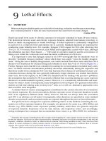
arsenic in tilapia (Oreochromis mossambicus) were estimated with a PBPK model in a recent study
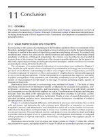
of human risk due to fish consumption (Ling et al. 2005) (Figure 8.3). These types of models, because
they originated in the medical sciences, are found most often in that part of the ecotoxicology liter-
ature focused on human exposure and risk from contaminants. As additional examples, Clewell and
Hearhart (2002) used PBPK models to estimate infant exposure to chemicals in breast milk. Yang
et al. (1998) included lipophilicity-based quantitative structure–activity relationships (QSARs) to
enrich current PBPK models of organic contaminant exposure.
8.2.7 S
TATISTICAL MOMENTS FORMULATIONS
The PBPK models just described are among the most complicated bioaccumulation models applied
by ecotoxicologists. At the other extreme are statistical methods that avoid explicit models yet

provide very useful information.
The classic statistical moments approach of Yamaoka et al. (1978) begins with a simple curve of
concentration (C
t
) in a compartment such as the blood or urine through time (t) after introduction of
© 2008 by Taylor & Francis Group, LLC
Clements: “3357_c008” — 2007/11/9 — 18:10 — page 126 — #12
126 Ecotoxicology: A Comprehensive Treatment
Gills
Blood
Muscle
Alimentary tract
Liver
Egestion
Metabolic
transformation
Growth
dilution
As input
from water
As exiting
gills chamber
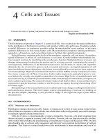
FIGURE 8.3 An example of a PBPK model. This figure depicts the compartment model used by Ling et al.
(2005) to predict arsenic accumulation in tilapia consumed by people inhabiting an area of Taiwan with high
incidence of arsenic poisoning (blackfoot disease). Dissolved arsenic passing over the gills can be taken up and
enter the circulation. Arsenic in the circulation can then accumulate in several tissues. It can also be diluted as
the fish grows (growth dilution), resulting in a decrease in concentration. It can be eliminated via the gut or
metabolism in the liver.
a substance, and estimates the zero to second moments of the curve:
AUC =


∞
0
C
t
dt, (8.31)
MRT =

∞
0
tC dt

∞
0
C dt
, (8.32)
VRT =

∞
0
(t − MRT)
2
C dt

∞
0
C dt
, (8.33)
where AUC (zero moment) =the area under the concentration–time curve, MRT = mean residence
time of the contaminant in the body, and VRT = the variance of the residence time. The MRT,

first moment of the concentration–time curve, is derived with the area under the curve of C × t
versus t, that is, the area under the moments curve (AUMC). The MRT is AUMC/AUC. It is the
time needed to eliminate 63.2% of the dose under the assumption of first order elimination (Gibaldi
1991). The AUC, MRT, and VRT are easily estimated from the C versus t data by methods described
by Yamaoka et al. (1978) and again by Newman (1995). Of course, if one specifies a model as done
in the methods described earlier, these moments can still be calculated. The unique aspect of this
approach is that a model is not required to produce useful information.
Several very useful metrics can be obtained with these methods. As an example, clearance after
intravenous (iv) injection can be estimated to be simply D
iv
/AUC (Medinsky and Klaassen 1996).
Also, if a dose was administered and the MRT calculated, the first order rate constant k
e
can be
estimated
k
e
=
1
MRT
. (8.34)
© 2008 by Taylor & Francis Group, LLC
Clements: “3357_c008” — 2007/11/9 — 18:10 — page 127 — #13
Models of Bioaccumulation and Bioavailability 127
The first order rate constant for absorption (k
a
) via the gut can be estimated from MRT val-
ues estimated if one administers a dose separately by iv (MRT
iv
) and then by ingestion (MRT

oral
)
(Gibaldi 1991)
MAT = MRT
oral
−MRT
iv
, (8.35)
where MAT is the mean absorption time of the chemical:
k
a
=
1
MAT
(8.36)
More will be made of statistical moments techniques in the next section.
8.3 BIOAVAILABILITY
Bioavailability is the extent to which a contaminant in a source is free for uptake. In many definitions,
especially those associated with pharmacology or mammalian toxicology, bioavailability of a contaminant
implies the degree to which the contaminant is free to be taken up and to cause an effect at the site of
action.
(Newman and Unger 2003)
8.3.1 CONCEPTUAL FOUNDATION:
C
ONCENTRATION→EXPOSURE→REALIZED DOSE→EFFECT
The foundation for the bioavailability concept is plain to see. The presence of a specified contaminant
concentration may or may not present a danger to an individual. Whether the organism is exposed to
the contaminant concentration will depend on whether it comes within close proximity of the media
containing the contaminant. The organism must be in appropriate contact in order to absorb, ingest,
imbibe, orinhale the contaminated material. Whether or notthiscontactresultsin a realized dose inthe

organism will depend on a wide range of factors that collectively determine bioavailability. We have
already discussed most of the important factors in previous chapters. If one defines bioavailability
in the restricted sense of availability to a site of action then toxicokinetics within the organism must
be considered. In such a case, assessment of bioavailability is concerned with predicting an effective
dose, i.e., the dose delivered to the site of action. To summarize, bioavailability is a metric for
translating contaminant exposure to a realized or effective dose. Its context may differ depending on
the researcher’s methods and intentions.
Box 8.3 What Is Involved in Oral Bioavailability?
Slightly differing terms and methods are used by ecotoxicologists and environmental risk
assessors to describe and study bioavailability of substances in food. Penry (1998) pointed
out that the processes of digestion, absorption, and assimilation all contribute to oral bioavail-
ability, but their contributions are often misunderstood and variable. This leads to confused
discussions of bioavailability and its measurement. Penry emphasizes how important it is
to understand the context in which “bioavailability” is discussed, providing the following
distinctions.
Digestion is the process by which ingested materials are broken down so that they are cap-
able of being absorbed across the gut lining. Digestion efficiency can be estimated by measuring
the amount of the substance in the ingested food (F
0
) and the amount of that same substance
© 2008 by Taylor & Francis Group, LLC
Clements: “3357_c008” — 2007/11/9 — 18:10 — page 128 — #14
128 Ecotoxicology: A Comprehensive Treatment
remaining in egested feces (F
e
):
Digestive efficiency = 1 −
F
e
F

0
. (8.37)
The next step, absorption, is the uptake of the products of digestion into cells of the gut
lining. Absorption efficiency reflects the fraction of the compound in the gut (F
g
) that passes
through the membranes of cells lining the gut lumen (F
c
):
Absorption efficiency = 1 −
F
c
F
g
. (8.38)
Assimilation involves the actual incorporation of the substance into the organisms’ tissues.
Assimilation efficiency is a measure of the fraction of total amount absorbed (F
a
) that is actually
assimilated into the tissues of the organism (F
t
):
Assimilation efficiency = 1 −
F
t
F
a
. (8.39)
According to Penry (1998), digestive and absorption efficiencies may be inappropri-
ately used as analogous to assimilation efficiency in many bioavailability studies. Obviously,

digestion, absorption, and assimilation all contribute to the realized bioavailability but each
is influenced by different processes that alone do not suffice to quantify bioavailability.
For example, selective sorting of particles by deposit feeders complicates estimation of diges-
tion efficiency, because some contaminant-containing particles will not be subject to digestive
processes, but instead, will simply pass out of the gut. And absorption does not necessarily
lead to assimilation. As discussed in the previous chapter, the uptake of benzo[a]pyrene by
cells of the gut, its conversion to benzo[a]pyrene-3-sulfate and benzo[a]pyrene-1-sulfate, and
consequent transport of these conjugates back into the gut lumen by ABC transport proteins
is one example of absorption into gut cells that does not result in direct delivery to the organ-
ism’s tissues for incorporation. Some substances can be metabolized in gut cells and fail to
move into circulation. Gibaldi (1991) provides several examples of drugs that undergo such
presystemic metabolism. Similarly, binding of contaminant entering the circulatory system and
rapid incorporation into bile can make it unavailable for assimilation into tissues. Finally, in
the context of delivery to the site of action, enterohepatic cycling of a substance would com-
plicate any simplistic use of digestion, absorption, or assimilation efficiencies alone to infer
bioavailability.
8.3.2 TYPES AND ESTIMATION OF BIOAVAILABILITY
Bioavailability is important to understand for dermal, inhalation, and ingestion routes although most
focus is on the ingestion route. Our previous discussions about dermal exposure and uptake from
water and air provide detail about the less commonly discussed routes. Often, bioavailability is
expressed as the fraction of the amount of the potentially available chemical that makes it into the
circulation or as the amount in a medium available for uptake based on some criterion. The first
expression will be used here.
Bioavailabilities can be either absolute or relative. TheAUC approach for ingested chemicals can
be used to illustrate absolute and relative bioavailability. The fraction (F) of an ingested dose (D)
that enters the circulation can be estimated as the AUC in the blood (or plasma) measured after
© 2008 by Taylor & Francis Group, LLC
Clements: “3357_c008” — 2007/11/9 — 18:10 — page 129 — #15
Models of Bioaccumulation and Bioavailability 129
ingestion (AUC

oral
) divided by the AUC measured after iv injection of the same dose (AUC
iv
):
F =
AUC
oral
AUC
iv
. (8.40)
In the above equation, the AUC estimated after iv administration is the reference AUC because
the availability of the iv administered dose is, by definition, 100%. Therefore, the F estimates the
fraction of the ingested dose that is available to reach the circulation. If the AUC increases linearly
with dose within the range being administered, an F can be calculated when the doses administered
intravenously and orally differ:
F =
AUC
oral
D
iv
AUC
iv
D
oral
. (8.41)
Similarly, relative bioavailabilities can be estimated with AUCs produced by administering doses
from two different sources. In this case, the AUC for one of the sources becomes the referenceAUC.
For example, AUCs can be estimated if a dose of a chemical was delivered in one type of food and
then in another:
F =

AUC
Food A
AUC
Food B
. (8.42)
In this example, the relative bioavailability indicates how much more or less a dose is available to
enter the circulation from the two different sources. Of course, other estimated parameters such as the
rate constants for absorption (Equation 8.36) from AUC analysis also suggest relative availabilities
for the ingested materials.
Box 8.4 Taking a Few Moments to Estimate Methylmercury Bioavailability
The accumulation of methylmercury in fish has become a major issue relative to human expos-
ure. Consequently, methylmercury bioaccumulation dynamics and bioavailability have become
important research themes. In methylmercury bioavailability studies using goldfish (Carassius
auratus) (Sharpe et al. 1977) and rainbow trout (O. mykiss) (Giblin and Massaro 1973),
the conventional mass balance approach was used to estimate bioavailability. Briefly, this
involves introducing a known amount of methylmercury in food, and after ample time passes
to allow unassimilated methylmercury to be eliminated from the body, measuring the amount
of methylmercury retained in the fish. This method can be compromised if the time needed to
remove unassimilated methylmercury is underestimated or if the elimination of the compound
of interest is very fast and a fraction of the assimilated methylmercury is eliminated before it
can be measured in the fish tissue.
McCloskey et al. (1998) applied AUC methods just described as a convenient means of
estimating oral methylmercury bioavailability to channel catfish (Ictalurus punctatus). Each
catfish was fitted with an aortic cannula that allowed blood samples to be taken through
time after dose administration. Each fish first received an oral methylmercury dose and the
time course of methylmercury in the blood was followed through time. The same catfish were
then given an intra-arterial dose and the time course of methylmercury concentration in the
blood followed again. The blood methylmercury concentrations were normalized to an average
hematocrit (17%) during computations because most of the methylmercury in the blood was
associated with the red blood cells and the hematocrit varied with time and among catfish.

© 2008 by Taylor & Francis Group, LLC
Clements: “3357_c008” — 2007/11/9 — 18:10 — page 130 — #16
130 Ecotoxicology: A Comprehensive Treatment
The dose-adjusted AUC approach (Equation 8.41) was applied to estimate oral bioavailab-
ility (F) for each catfish, using both noncompartment and compartment model–based methods.
The noncompartment-based method simply used the linear trapezoidal method to measure
AUC. The compartment model involved fitting of a triexponential model for the intra-arterial
injected dose
C
blood,t
= Ae
−πt
+Be
−αt
+Ce
−βt
and estimating the AUC as
AUC
0→∞
=
A
π
+
B
α
+
C
β
.
A more involved model with a lag time before gut absorption of the dose (D) and a biex-

ponential decline in blood concentrations was used for the orally administered dose. The blood
methylmercury concentration was modeled under the assumption that it exchanged by first
order kinetics between central and peripheral compartments (k
21
), and gut absorption could be
defined with a first order rate constant (k
a
) after an initial lag (lag) of approximately 4 h before
absorption:
C
blood,t
=k
a
D

F
V
central


(k
21
−α)e
−α(t−lag)
(k
a
−α)(β − α)
+
(k
21

−β)e
−β(t−lag)
(k
a
−β)(α − β)
+
(k
21
−k
a
)e
−k
a
(t−lag)
(α −k
a
)(β −k
a
)

.
The F and V
central
in this model are the bioavailability and volume of the central compartment,
respectively.
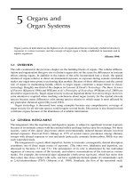
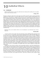
Figure 8.4 shows the bioavailabilities (F) estimated with both approaches. The first point to
make from this plot is that bioavailability is strongly influenced by feeding rates. Bioavailability
was highest for fish receiving the least amount of food. Also, the compartment model method
gave similar, but slightly lower, estimates of bioavailability as the noncompartmental method.
FIGURE 8.4 Bioavailability (F) estimated for

methylmercury fed to channel catfish in vary-
ing amounts of food. The AUC estimates were
generated with two methods (model free and a
model-based method) (McCloskey et al. 1998).
Bioavailability (F )
0.0
0.6
0.1
0.2
0.3
0.4
0.5
Amount of food gavaged (g/kg of fish)
5
0
10 15 20 25
Noncompartment
method
Compartment
model method
Bioavailability can be estimated in other ways. As mentioned above, the amount of a delivered
dose that becomes incorporated in the tissues or not egested has been used to estimate bioavailability.
Bias can emerge in such an estimated bioavailability if the compound is eliminated very quickly
so that a significant amount of the compound making it to the circulation is lost during the time that
one is waiting for the unassimilated contaminant in the gut to clear. An opposite bias can emerge
if insufficient time is allowed for gut clearance and unassimilated contaminant in the gut is incor-
rectly included in estimates of that incorporated into the organism’s tissues. A dual-isotope approach
© 2008 by Taylor & Francis Group, LLC
Clements: “3357_c008” — 2007/11/9 — 18:10 — page 131 — #17
Models of Bioaccumulation and Bioavailability 131

can be used to minimize the risk of having unassimilated chemical in the organism’s system at
the time chosen to estimate F. Reinfelder and Fisher (1991) used such a method to estimate F for
a series of metals in food fed to marine copepods. An inert (notionally unavailable) radionuclide
tracer such as
51
Cr is incorporated into the food along with a radioactive form of the chemical
of interest (e.g.,
65
Zn). The assumption is made that both radionuclides are similarly incorpor-
ated into the food. The dual-labeled food is given to the organism and the radioactivity associated
with the inert tracer measured until it has been completely eliminated, indicating that unassimil-
ated material has passed from the organism by that time. The amount of the other chemical of
interest (e.g.,
65
Zn) that remains in the organism at that point is used to estimate F. This general
method has been extremely useful and can be modified even if a completely inert tracer is not avail-
able. The dual-labeled isotope approach can be biased if the inert tracer is not incorporated into
the food identically to the element/chemical for which F is being estimated. Lydy and Landrum
(1993) provide one example in which
51
Cr was not incorporated into sediment similarly to the
toxicant of interest (benzo[a]pyrene). In combination with the selective feeding by Diporeia spp.,
heterogeneous labeling produced unacceptable estimates of bioavailability. Instead, estimation for
sediment-associated [
14
C]benzo[a]pyrene required a mass-balance approach with carbon normaliz-
ation. Total organic carbon and [
14
C]benzo[a]pyrene were determined in fecal pellets and sediment
from the exposure systems. A selectivity index (SI) was estimated in order to calculate F in the

presence of selective feeding on sediment particles.
SI =
[TOC
feces
/(1 − RC)]
TOC
sediment
, (8.43)
where TOC
feces
and TOC
sediment
are TOC fraction of the feces or sediment, respectively, and
RC is the fractional loss of carbon during passage through the gut as obtained from the literat-
ure in this case. The assimilation of benzo[a]pyrene could then be calculated using the following
equation:
F =
SI ×C
sediment
−C
feces
SI ×C
sediment
. (8.44)
Another means of estimating F in such a situation is to use SI and feeding rates, as done by
Kukkonen and Landrum (1995) in their assessment of assimilation of sediment-associated PAH
and PCB congeners.
8.4 SUMMARY
In this chapter, the basic quantitative approaches applied to bioaccumulation were described as well
as the basic approaches to estimating bioavailability. Rate constant-, clearance-, and fugacity-based

formulations were described. Many of these methods can be used to generate simple or complex
PBPK models. Fugacity-based models have a distinct advantage relative to the major goal of this
book of fostering consilience amonglevels of complexity. The concept of bioavailability andmethods
for its estimation were also explored.
8.4.1 SUMMARY OF FOUNDATION CONCEPTS AND PARADIGMS
• Bioaccumulation can be modeled with rate constant-, clearance-, and fugacity-based
formulations.
• The kinetics associated with the bioaccumulation process are most often described using
first or mixed order (saturation) formulations although other reaction orders are possible.
© 2008 by Taylor & Francis Group, LLC
Clements: “3357_c008” — 2007/11/9 — 18:10 — page 132 — #18
132 Ecotoxicology: A Comprehensive Treatment
• Bioaccumulation models can describe mathematical compartments/processes or physical
compartments/processes as in the case of PBPK (or PBTK) models.
• Noncompartment statistical moments methods can also generate extremely useful
information about bioaccumulation processes and bioavailability.
• Procedures used to estimate bioavailability vary. Each method has advantages and slight
differences, making it important to understand fully what each actually indicates.
• Bioavailabilities can be described as absolute or relative depending on the purpose of the
associated study.
REFERENCES
Anderson, P.D. and Spear, P.A., Copper pharmacokinetics in fish gills—I. Kinetics in pumpkinseed sunfish,
Lepomis gibbosus, of different body size, Water Res., 14, 1101–1105, 1980.
Buchwalter, D.B., Jenkins, J.J., and Curtis, L.R., Temperature influences on water permeability and chlorpyrifos
uptake in aquatic insects with differing respiratory strategies, Environ. Toxicol. Chem., 22, 2806–2812,
2003.
Bury, N.R., Grosell. M., Grover, A.K., and Wood, C.M., ATP-dependent silver transport across the basolateral
membrane of rainbow trout gills, Toxicol. Appl. Pharmacol., 159, 1–8, 1999.
Clewell, R.A. and Gearhart, J.M., Pharmacokinetics of toxic chemicals in breast milk: Use of PBPK models to
predict infant exposure, Environ. Health Perspect., 110, A333–A337, 2002.

Czub, G. and McLachlan, M.S., A food chain model to predict the levels of lipophilic organic contaminants in
humans, Environ. Toxicol. Chem., 23, 2356–2366, 2004.
Erickson, R.J. and McKim, J.M., A model of exchange of organic chemicals at fish gills: Flow and diffusion
limitations, Aquat. Toxicol., 18, 175–198, 1990.
Gibaldi, M. Biopharmaceutics and Clinical Pharmacokinetics, 4th ed., Lea and Febiger, Ltd., Malvern, PA,
1991, p. 406.
Giblin, F.J. and Massaro, E.J., Pharmacodynamics of methyl mercury in the rainbow trout (Salmo gairdneri):
Tissue uptake, distribution and excretion, Toxicol. Appl. Pharmacol., 24, 81–91, 1973.
Gobas, F.A.P.C. and Mackay, D., Dynamics of hydrophobic organic chemical bioconcentration in fish, Environ.
Toxicol. Chem., 6, 493–504, 1987.
Haddad, S. and Krishnan, K., Physiological modeling of toxicokinetic interactions: Implications for mixture
risk assessment, Environ. Health Perspect., 106, 1377–1384, 1998.
Hickie, B.E., Mackay, D., and de Koning, J., Lifetime pharmacokinetic model for hydrophobic contaminants
in marine mammals, Environ. Toxicol. Chem., 18, 2622–2633, 1999.
Kukkonen, J. and Landrum, P.F., Measuring assimilation efficiencies for sediment-bound PAH and PCB
congeners by benthic organisms, Aquat. Toxicol., 32, 75–92, 1995.
Ling, M P., Liao, C M., Tsai, J W., and Chen, B C.,APBTK/TD modeling-based approach can assess arsenic
bioaccumulation in farmed Tilapia (Oreochromis massambicus) and human health risks, Int. Environ.
Assess. Man., 1, 40–54, 2005.
Lydy, M.J. and Landrum, P.F., Assimilation efficiency for sediment-sorbed benzo[a]pyrene by Diporeia spp.,
Aquat. Toxicol., 26, 209–224, 1993.
Mackay, D., Finding fugacity feasible, Environ. Toxicol. Chem., 13, 1218–1223, 1979.
Mackay, D., Multimedia Environmental Models: The Fugacity Approach, 2nd ed., CRC Press/Lewis Publishers,
Boca Raton, FL, 2001, p. 272.
Mackay, D., Peterson, S., Cheung, B., and Neely, W.B., Evaluating the environmental behavior of chemicals
with a Level III fugacity model, Chemosphere, 14, 335–374, 1985.
Mackay, D. and Wania, F., Transport of contaminants to theArctic: Partitioning, processes and models, Sci. Total
Environ., 160/161, 25–38, 1995.
McCloskey, J.T., Schultz, I.R., and Newman, M.C., Estimating the oral bioavailability of methylmercury in
channel catfish (Ictalurus punctatus), Environ. Toxicol. Chem., 17, 1524–1529, 1998.

Medinsky, M.A. and Klaassen, C.D., Toxicokinetics, In Casarett & Doull’s Toxicology. The Basic Science of
Poisons, Klaassen, C.D. (ed.), McGraw-Hill, New York, 1996, pp. 187–198.
Newman, M.C., Quantitative Methods in Aquatic Ecotoxicology, CRC Press/Lewis Publishers, Boca Raton,
FL, 1995, p. 426.
© 2008 by Taylor & Francis Group, LLC
Clements: “3357_c008” — 2007/11/9 — 18:10 — page 133 — #19
Models of Bioaccumulation and Bioavailability 133
Newman, M.C. and Unger, M.A., Fundamentals of Ecotoxicology, CRC Press/Lewis Publishers, Boca Raton,
FL, 2003.
Nichols, J.W., McKim, J.M., Andersen, M.E., Gargas, M.L., Clewell, H.J., III, and Erickson, R.J., A physiolo-
gically based toxicokinetic model for the uptake and disposition of waterborne organic chemicals in
fish, Toxicol. Appl. Pharmacol., 106, 433–447, 1990.
Nichols, J.W., McKim, J.M., Lien, G.J., Hoffman,A.D., and Bertelsen, S.L., Physiologicallybased toxicokinetic
modeling of three waterborne chloroethanes in rainbow trout (Oncorhynchus mykiss), Toxicol. Appl.
Pharmacol., 110, 374–389, 1991.
Penry, D.L., Applications of efficiency measurements in bioaccumulation studies: Definitions, clarifications,
and a critique of methods, Environ. Toxicol. Chem., 17, 1633–1639, 1998.
Piszkiewicz, D., Kinetics of Chemical and Enzyme-Catalyzed Reactions, Oxford University Press, New York,
1977, p. 235.
Raaijmakers, J.G.W., Statistical analysis of the Michaelis–Menten equation, Biometrics, 43, 793–803, 1987.
Reinfelder, J.R. and Fisher, N.S., The assimilation of elements ingested by marine copepods, Science, 251,
794–796, 1991.
Sharpe, M.S., DeFreitas, A.S.W., and McKinnon, A.E., The effect of body size on methylmercury clearance by
goldfish (Carassius auratus), Environ. Biol. Fish., 2, 177–183, 1977.
Teorell, T., Kinetics of distribution of substances administered to the body. I. The extravascular modes of
administration, Arch. Int. Pharmacodyn., 57, 205–225, 1937a.
Teorell, T., Kinetics of distribution of substances administered to the body. I. The intravascular modes of
administration, Arch. Int. Pharmacodyn., 57, 226–240, 1937b.
Wagner, J.G., Fundamentals of Clinical Pharmacokinetics, Drug Intelligence Publications, Hamilton, IL, 1979,
p. 461.

Wania, F. and Mackay, D., A global distribution model for persistent organic chemicals, Sci. Total Environ.,
160/161, 211–232, 1995.
Wania, F., Mackay, D., Li, Y F., Bidleman, T.F., and Strand, A., Global chemical fate of
α-hexachlorocyclohexane. I. Evaluation of a global distribution model, Environ. Toxicol. Chem.,
18, 1390–1399, 1999.
Yamaoka, Y., Nakagawa, T., and Uno, T., Statistical moments in pharmacokineties, J. Pharmaco. Biopharmac.,
6-6, 547–558, 1978.
Yang, R.S.H., Thomas, R.S., Gustafson, D.L., Campain, J., Benjamin, S.A., Verhaar, H.J.M., and
Mumtaz, M.M., Approaches to developing alternative and predictive toxicology based on PBPK/PD
and QSAR modeling, Environ. Health Perspect., 106, 1385–1393, 1998.
Yang, R., Thurston, V., Neuman, J., and Randall, D.J.,Aphysiological model to predict xenobiotic concentration
in fish, Aquat. Toxicol., 48, 109–117, 2000.
© 2008 by Taylor & Francis Group, LLC