ECOTOXICOLOGY: A Comprehensive Treatment - Chapter 14 pot

Clements: “3357_c014” — 2007/11/9 — 12:42 — page 241 — #1
14
Toxicants and Simple
Population Models
14.1 TOXICANTS EFFECTS ON POPULATION SIZE
AND DYNAMICS
14.1.1 T
HE POPULATION-BASED PARADIGM FOR
ECOLOGICAL RISK
The greatest scandal of philosophy is that, while around us the world of nature perishes philosophers
continue to talk, sometimes cleverly and sometimes not, about the question of whether this world exists.
(Popper 1972)
Every scientific discipline is built around a collection of conceptual and methodological paradigms
that are “revealed in its textbooks, lectures, and laboratory exercises” (Kuhn 1962). These paradigms
define what the discipline encompasses—and what it does not. During professional training, a scient-
ist also learns the rules by which business within his or her discipline is to be conducted. A scientist
understands that there is a “hard core” of irrefutable beliefs that are not to be questioned and a
“protective belt of auxiliary hypotheses” that are actively tested and enriched (Lakatos 1970). To
venture outside the accepted borders of a discipline or to question a core paradigm is courting pro-
fessional censure. Yet, when a core paradigm fails too obviously and another is available to take
its place, significant shifts do occur in a discipline. Oddly enough, a clearly inadequate paradigm
will remain central in a discipline if a better one is not available to replace it (Braithwaite 1983).
Because scientists are human, the shift from one core paradigm to another is characterized by as
much discomfort and bickering as excitement.
Although originating from illogical roots, the dogmatic tendency to cling to a paradigm does
have a positive consequence (Popper 1972). Any group of scientists who tends to drop a central
paradigm too quickly will experience many disappointments and false starts. Akey character of any
scientific discipline is a healthy, not pathological, tenacity of central paradigms.
In writing this and several of the remaining chapters, we are caught between the risk of being
censured for discussing topics out of balance with their perceived importance in ecotoxicology and
the conviction that, until recently, ecotoxicologists have been dawdling in accepting a useful, new

core paradigm for evaluating ecological effects. Much like the negligent philosophers described in
the quote above, ecotoxicologists were enjoying the exploration of the innumerable details of their
protective belt of auxiliary paradigms and hypotheses while important questions remained poorly
addressed by an individual-based paradigm. Fortunately, ecotoxicologists are now focusing much
more on population-based metrics of effect. It is obvious that prediction of population consequences
cannot be adequately done by simply modifying the present individual-based metrics. Instead of
adding to the protective belt around this collapsing paradigm, ecotoxicologists are now producing
more population-level metrics of effects.
What is needed is even more effort to clearly articulate a new population-based paradigm. Also,
nontraditional methods must be explored carefully in order to generate a belt of auxiliary hypo-
theses around this new population-based paradigm. Since the early 1980s (e.g., Moriarty 1983),
the argument for population-based methods taking precedence over individual-based metrics of
241
© 2008 by Taylor & Francis Group, LLC
Clements: “3357_c014” — 2007/11/9 — 12:42 — page 242 — #2
242 Ecotoxicology: A Comprehensive Treatment
effect has been voiced with increasing frequency in scientific publications, regulatory documents,
and federal legislation. Recently, Forbes and Calow (1999) reiterated this theme and provided
more evidence to support it by comparing individual- and population-based metrics for ecolo-
gical impact assessment. Also, individual-based models for populations (e.g., DeAngelis and Gross
1992) have emerged to bridge the gap between individual- and population-based metrics for judging
ecological risk.
14.1.2 EVIDENCE OF THE NEED FOR THE POPULATION-BASED
PARADIGM FOR RISK
The quotes below are chosen to reflect the transition taking place in our thinking about ecotox-
icological risk assessment. Early quotes point to the underutilization of population-based metrics
of toxicant effect. The need for more population-based predictions is then expressed in a series of
regulation-oriented publications. Finally, statements made during the past few years show that meth-
ods are now available and are being applied with increasing frequency to address population-level
questions.

Ecologists have used the life tablesince its introduction by Birch (1948) to assess survival, fecundity, and
growth rate of populations under various environmental conditions. While it has proved a useful tool in
analyzing the dynamics of natural populations, the life table approach has not, with few exceptions ,
been used as a toxicity bioassay.
(Daniels and Allan 1981)
There is an enormous disparity between the types of data available for assessment and the types of
responses of ultimate interest. The toxicological data usually have been obtained from short-term tox-
icity tests performed using standard protocols and test species. In contrast, the effects of concern to
ecologists performing assessments are those of long-term exposures on the persistence, abundance,
and/or production of populations.
(Barnthouse 1987)
Environmental policy decision makers have shifted emphasis from physiological, individual-level to
population-level impacts of human activities. This shift has, in turn, spawned the need for models of
population-level responses to such insults as contamination by xenobiotic chemicals.
(Emlen 1989)
Protecting populations is an explicitly stated goal of several Congressional and Agency mandates and
regulations. Thus it is important that ecological risk assessment guidelines focus upon protection and
management at the population, community, and ecosystem levels
(EPA 1991)
The Office of Water is required by the Clean Water Act to restore and maintain the biological integrity of
the nation’s waters and, specifically, to ensure the protection and propagation of a balanced population
of fish, shellfish, and wildlife.
(Norton et al. 1992)
The translation from a pollutant’s effects on individuals to its effects on the population can be
accomplished using life-history analysis to calculate the effect on the population’s growth rate.
(Sibly 1996)
In this chapter, I am concerned with the translation from individuals to populations using demographic
models as a link. Individual organisms are born, grow, reproduce and die, and exposure to toxicants alters
the risks of these occurrences. The dynamics of populations are determined by the rates of birth, growth,
© 2008 by Taylor & Francis Group, LLC

Clements: “3357_c014” — 2007/11/9 — 12:42 — page 243 — #3
Toxicants and Simple Population Models 243
fertility, and mortality that are produced by these individual events . By incorporating individual
rates into population models, the population effects of toxicant-induced changes in those rates can be
calculated.
(Caswell 1996)
Fortunately, traditional populationand demographic analysescan be used topredict the possibleoutcomes
of exposure and their probabilities of occurring. Although most toxicity testing methods do not produce
information directly amenable to demographic analysis, some ecotoxicologists have begun to design
tests and interpret results in this context.
(Newman 1998)
Our conclusion is that r [the population growth rate] is a better measure of responses to toxicants than are
individual-level effects, because it integrates potentially complex interactions among life-history traits
and provides a more relevant measure of ecological impact.
(Forbes and Calow 1999)
What is needed is a complete understanding of these approaches and their merits, and the resolve to
move further to this new context. As suggested in the above quote by Caswell (1996), individual-
based information can be used to assess population-level effects if individual-based metrics are
produced with translation to the population level in mind. Valuable time and effort are wasted if
we are not mindful of the need for hierarchical consilience. Sufficient understanding will foster
the generation of more population-based data and its eventual application in routine ecological risk
assessments. It will also foster the infusion of methods from disciplines such as conservation biology,
fisheries and wildlife management, and agriculture that have similar goals and relevant technologies.
Toward these ends, this and the next chapter will build a fundamental understanding of population
processes. Some supporting detail including methods for fitting data to these models can be found
in Newman (1995).
14.2 FUNDAMENTALS OF POPULATION DYNAMICS
14.2.1 G
ENERAL
Initially, we assume that a population is composed of similar individuals occupying a spatially uni-

form habitat. Because the qualities of individuals are lost in models with such assumptions, they are
often called phenomenological models—models focused on describing a phenomenon but not linked
intimately to causal mechanics (i.e., not mechanistic models). Events occurring in individuals such as
birth, growth, reproduction, and death are aggregated into summary statistics such as population rate
of increase. Exploration of these models creates an understanding of population behaviors possible
under different conditions. However, without details for individuals and inclusion of interactions
with other species populations, insights derived from these models should not be confused with cer-
tain knowledge. The problem of ecological inference may appear if results are used to imply behavior
of individuals. Alternatively, if results were applied to predicting population fate in a contaminated
ecosystem, problems may arise because an important emergent property might have been overlooked
(e.g., see Box 16.1).
Modeled populations can display continuous or discrete growth dynamics depending on the
species and habitat characteristics in question. Continuous growth dynamics are anticipated for a
species with overlapping generations and discrete growth dynamics are anticipated for species with
nonoverlapping generations. Nonoverlapping generations are common for many annual plant or
insect populations. Continuous and discrete growth dynamics are described below with differential
and difference equations, respectively. Some of the differential models will also be integrated to
allow prediction of population size through time.
© 2008 by Taylor & Francis Group, LLC
Clements: “3357_c014” — 2007/11/9 — 12:42 — page 244 — #4
244 Ecotoxicology: A Comprehensive Treatment
14.2.2 PROJECTION BASED ON PHENOMENOLOGICAL MODELS:
C
ONTINUOUS GROWTH
The change in size (N) of a population experiencing unrestrained, continuous growth is described
by the differential equation
dN
dt
= bN −dN = (b −d)N = rN, (14.1)
where r = the intrinsic rate of increase or per capita growth rate. The r parameter is the difference

between the overall birth (b) and death (d) rates (Birch 1948). Obviously, population numbers
decline if b < d (i.e., r < 0) or increase if b > d (i.e., r > 0). Integration of Equation 14.1
yields Equation 14.2 and allows estimation of population size at any time based on r and the initial
population size, N
0
,
N
t
= N
0
e
rt
. (14.2)
The amount of time required for the population to double (population doubling time, t
d
) is (ln 2)/r.
This model may be applicable for some situations such as the early growth dynamics of a
population introduced into a new habitat or a Daphnia magna population maintained in a laboratory
culture with frequent media replacement. However, most habitats have a finite capacity to sustain
the population. This finite capacity slowly comes to have a more and more important role in the
growth dynamics as the population size increases. The change in number of individuals through time
slows as the population size approaches the maximum size sustainable by the habitat (the carrying
capacity or K). This occurs because b −d is not constant through time. Birth and death rates change
as population size increases. More than 150 years ago, Verhulst (1838) accommodated this density
dependence with the term 1−(N/K) producing the logistic model for population density-dependent
growth in the following equation:
dN
dt
= rN


1 −
N
K

. (14.3)
The per capita growth rate (r
dd
= r[1 −(N/K)]) is now dependent on the population density.
As population size increases, birth rates decrease and death rates increase. These rates are b =
b
0
− k
b
N and d = d
0
+ k
d
N where b
0
and d
0
are the nearly density-independent birth and death
rates experienced at very low population densities. The terms k
b
and k
d
are slopes for the change in
birth and death rates with change in population density. The logistic model can be expressed in these
terms (Wilson and Bossert 1971),
dN

dt
=[(b
0
−k
b
N) −(d
0
+k
d
N)]N. (14.4)
The carrying capacity (K) can also be expressed in these terms, K =[(b
0
− d
0
)/(k
b
+ k
d
)]
(Wilson and Bossert 1971).
The model described by Equation 14.3 carries the assumption that there is no delay in population
response, that is, there is an instantaneous change in r
dd
due to any change in density. A delay (T)
can be added to Equation 14.3:
dN
dt
= rN

1 −

N
t−T
K

. (14.5)
© 2008 by Taylor & Francis Group, LLC
Clements: “3357_c014” — 2007/11/9 — 12:42 — page 245 — #5
Toxicants and Simple Population Models 245
Time
Number of individuals
K
θ
2
θ
1
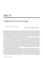
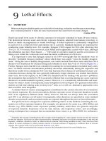
FIGURE 14.1 Logistic increase with population growth symmetry being influenced by the θ parameter in the
θ-Ricker model (Equation 14.7).
A time lag (g) before the population responds favorably to a decrease in density can also be
included. Such a lag might be applied for species populations in which individuals must reach a
certain age before they are sexually mature:
dN
dt
= rN
t−g

1 −
N
t−T
K


. (14.6)
Gilpin and Ayala (1973) found that the shape of the logistic model was not always the same for
different populations and added a term (θ ) to Equation 14.3 to make the logistic model more flexible.
This flexible model (Equation 14.7) is called the θ-logistic model (Figure 14.1):
dN
dt
= rN

1 −

N
K

θ

. (14.7)
Obviously, delays could be placed into Equation 14.7, if necessary, to produce a model of density-
dependent growth for a population with time lags in responding to density changes, continuous
growth, and growth symmetry defined by θ.
A density-independent effect (I) on population growth such as that of a toxicant can be added to
Equation 14.3:
dN
dt
= rN

1 −
N
K

−I. (14.8)

The I canalso beexpressed assome toxicant-related “loss,” “take,” or“yield” fromthe population
at anymoment (E
Toxicant
N), whereE
Toxicant
is theproportion of the existing number of individuals(N)
taken owing to toxicant exposure
dN
dt
= rN

1 −
N
K

−E
Toxicant
N. (14.9)
In words, this model predicts the change in number of individuals per unit of time as a function
of the intrinsic rate of increase, density-dependent growth dynamics, and a density-independent
decrease in numbers of individuals as a result of toxicant exposure. In this form, it is identical to
a rudimentary harvesting model for natural populations (e.g., commercial fish harvesting) and is
amenable to analysis of population sustainability and recovery (see Everhart et al. 1953, Gulland
1977, Hadon 2001, Murray 1993). The difference is that harvesting involves toxicant action instead
of fishing. We will discuss this point later, but it is important now to realize that toxicant-induced
changes inK, r, T, g, andθ are possible andnone ofthese parametersshould be ignored in the analysis
© 2008 by Taylor & Francis Group, LLC
Clements: “3357_c014” — 2007/11/9 — 12:42 — page 246 — #6
246 Ecotoxicology: A Comprehensive Treatment
of population fate with toxicant exposure. If necessary to produce a realistic model, time delays and

θ values can be added to Equation 14.8. The underlying processes resulting in these delays could
be influenced by toxicant exposure. For example, a toxicant may influence the time required for an
individual to reach sexual maturity.
Prediction of population size through time for density-dependent growth of a population with
continuous growth dynamics and no time delays is usually done using Equations 14.10 or 14.11.
These equations are different forms of the sigmoidal growth model. May and Oster (1976) provide
other useful forms:
N
t
=
N
0
K e
rt
K + N
0
(e
rt
−1)
(14.10)
N
t
=
K
1 +[(K − N
0
)/N
0
]e
−rt

(14.11)
Newman (1995) describes methods for fitting data to these differential and integrated equations
and relates them to ecotoxicology.
14.2.3 PROJECTION BASED ON PHENOMENOLOGICAL MODELS:
D
ISCRETE GROWTH
Unrestrained growth of populations displaying discrete growth (nonoverlapping generations) is
described with the difference equation,
N
t+1
= λN
t
, (14.12)
where N
t
and N
t+1
are the population sizes at times t and t +1 respectively, and λ is the finite rate of
increase, which can be related to r (intrinsic or infinitesimal rate of increase) with Equation 14.13.
It is the number of times that the population multiplies in a time unit or step (Birch 1948). The
time step may be arbitrary (e.g., time between census episodes) or associated with some aspect of
reproduction (e.g., time between annual calvings):
λ =
N
t+1
N
t
= e
r
. (14.13)

The characteristicreturn time (T
r
) canbe estimated from r orλ. It isthe estimatedtime requiredfor
a population changing in size through time to return toward its carrying capacity or, more generally,
toward its steady state number of individuals (May et al. 1974). It is the inverse of the instantaneous
growth rate, r (i.e., T
r
= 1/r). The T
r
gets shorter as the growth rate, r, increases: faster growth
results in a faster approach toward steady state. In Section 4.3, the influence of T
r
on population
stability will be described.
This difference equation (Equation 14.12) can be expanded to include density-dependence
using several models (see Newman 1995). Equations 14.14 and 14.15 are the classic Ricker and
a modification of it that includes Gilpin’s θ parameter (the θ-Ricker model), respectively:
N
t+1
= N
t
e
r(1−(N
t
/K))
(14.14)
N
t+1
= N
t

e
r[1−(N
t
/K)
θ
]
. (14.15)
As done with the differential models, we have accommodated differences in growth curve sym-
metry by including a θ term in Equation 14.15. But what about adding lag terms? Because the form of
the difference equations implies an inherent lag from t to t +1, these models may not need additional
© 2008 by Taylor & Francis Group, LLC
Clements: “3357_c014” — 2007/11/9 — 12:42 — page 247 — #7
Toxicants and Simple Population Models 247
terms to accommodate lags. If a lag time different from the time step (t to t + 1) is required, it can
be added by using N
t−1
, N
t−2
, or some other past population size instead of N
t
where appropriate
in these models. We can add an effect of a density-independent factor such as toxicant exposure
to the logistic model. The difference models above are modified by inserting an I term as done
in Equations 14.8 and 14.9. The modification made by Newman and Jagoe (1998) to the simplest
difference model (Equation 4.16) is provided as follows (Equations 4.17 and 4.18).
N
t+1
= N
t


1 +r

1 −
N
t
K

(14.16)
N
t+1
= N
t

1 +r

1 −
N
t
K

−I (14.17)
N
t+1
= N
t

1 +r

1 −
N

t
K

−E
Toxicant
N
t
(14.18)
I is the number of individuals “taken” from the parental population by the toxicant at each time step.
Again, these models of toxicant effect are comparable to those used to manage harvested, renewable
resources such as a fishery [e.g., Equations 2.13 and 2.15 in Haddon (2001)]. Alternately, Gard
(1992) expresses the influence of a toxicant directly in terms of the instantaneous growth rate (r)at
time, t,
r
t
= r
0
−r
1
C
T(t)
, (14.19)
where r
0
is the intrinsic rate of increase in the absence of toxicant, C
T(t)
is a time-dependent effect of
the toxicant on the population, and r
1
is a units conversion parameter. Gard’s model is composed of

three differential equations that link temporal changes in environmental concentrations of a toxicant,
concentrations in the organism, and population growth (Gard 1990). At this point, it is only necessary
to note that Gard’s equations reduce r directly as a consequence of toxicant exposure. Any change
in r can influence population stability, as we will see in Section 14.3.
14.2.4 SUSTAINABLE HARVEST AND TIME TO RECOVERY
The expressions of toxicant-impacted population growth described to this point are equivalent to
those general models explored by Murray (1993) for population harvesting. Therefore, his expansion
of associated mathematicsand explanationsare translated directlyin thissection intotermsof toxicant
effects on populations. Let us assume that natality is not affected but the loss of individuals from the
population is affected by toxicant exposure. For the differential model (Equations 14.8 and 14.9),
Murray defines a harvest or yield that is analogous to I in Equation 14.8 and a corresponding new
steady-state population size of N
h
. This harvest is equivalent to E · N where E is a measure of the
harvesting intensity and N is the size of the population being harvested. The E is identical by intent
to E
Toxicant
in Equation 14.9. With “harvesting” or loss upon toxicant exposure, the population will
not have a steady-state size of K. Instead, it will have the following steady-state size if r is larger
than E
Toxicant
,
N
L
= K

1 −
E
Toxicant
r


, (14.20)
where N
L
is equivalent to Murray’s N
h
except that loss is now due to toxicant exposure. From
Equation 14.20, it is clear that the population at steady state will drop to zero if the intensity of the
toxicant effect (E
Toxicant
) is equal to or greater than r.
© 2008 by Taylor & Francis Group, LLC
Clements: “3357_c014” — 2007/11/9 — 12:42 — page 248 — #8
248 Ecotoxicology: A Comprehensive Treatment
Let us extend Murray’s expression of yield from a harvested population in order to gain further
insight into the loss that a population can sustain from toxicant exposure without being irreparably
damaged. The yield in Murray’s Equation 1.43 is modified to Equation 14.21 in order to define the
loss of individuals (L) expected at a certain intensity of effect (E
Toxicant
),
L
E
Toxicant
= E
Toxicant
K

1 −
E
Toxicant

r

. (14.21)
In words, the population loss or “yield” due to toxicant exposure (L
E
Toxicant
) is the new carrying
capacity (N
L
) multiplied by the E
Toxicant
: the yield is the number of individuals available to be taken
times the toxicant-induced fraction “taken.” Applying Equation 14.21, rK/4 is the maximum sustain-
able loss to toxicant exposure (analogous to the maximum sustainable yield where E
Toxicant
= r/2).
The new steady-state population size (N
L
, equivalent to N
h
) will be K/2 at this point of maximum
sustainable loss or “yield.” The population is growing maximally under these conditions. Population
growth becomes suboptimal if E
Toxicant
increases further and may even become negative if E
Toxicant
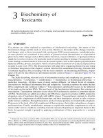
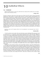
exceeds r. Figure 14.2 illustrates this general estimation of toxicant take or loss for a hypothetical
population that is growing according to the logistic model.
Moriarty (1983) makes several important points regarding this approach to analyzing toxicant
effectson populations. First, growthmeasured asa changein numberbetween times t and t+1 willnot

necessarily decrease with increasing loss from the population due to toxicant exposure (Figure 14.2).
It might increase. Surplus young produced in populations allows a certain level of mortality without
an adverse affect on population viability. Different populations have characteristic ranges of loss that
can be accommodated. Low losses potentially increase the rate at which new individuals appear in a
population and high losses push the population toward local extinction. Second, the carrying capacity
of the population will decrease as losses due to toxicant exposure increase. Third, there can be two
population sizes that produce a particular yield on either side of the N
t
for maximum yield. Increases
Population size at time, t (N
t
)
Population size at time,
t + 1 (N
t +1
)
N
t
= N
t + 1
Predictions from
logistic model
FIGURE 14.2 The maximum sustainable yield can be visualized by comparing the curve for the population
size at time steps N
t
and N
t+1
to the line for N
t
= N

t+1
. The population is not changing from one time to
another along the line for N
t
= N
t+1
, i.e., the population is at steady state. The vertical distance between the
curve of population size at time steps N
t
and N
t+1
and the line for N
t
= N
t+1
defines the sustainable yield
resulting from surplus production in the population each time step. The vertical dashed line shows the yield
that is maximal for this population. The reader is encouraged to review Waller et al. (1971) as an example of
using this type of curve with zinc-exposed fathead minnow (Pimephales promelas) populations. (Modified from
Figure 2.11 of Moriarty (1983) and Figure 2.2a of Murray (1993).)
© 2008 by Taylor & Francis Group, LLC
Clements: “3357_c014” — 2007/11/9 — 12:42 — page 249 — #9
Toxicants and Simple Population Models 249
or decreases in toxicant exposure can produce the same results in the context of population change.
Failure to recognize this possibility could lead to muddled interpretation of results from monitoring
of populations in contaminated habitats. An important advantage of the sustainable yield context
just developed is a more complete understanding of population consequences at various intensities
of loss due to toxicant exposure.
There is another advantage to ecotoxicologists taking an approach used by renewable resource
managers. Often, ecological risk assessments focus on recreational or commercial species, for

example, consequences of toxicant exposure to a salmon or blue crab fishery. Expressing toxic-
ant effects to populations with the same equations used by fishery or wildlife managers attempting
to regulate annual harvest allows simultaneous consideration of losses from fishing and pollution.
Another characteristic of harvested populations that is useful to the ecotoxicologist is the time to
recovery. The time to recover (return to an original population size) after harvest can be estimated in
terms of loss due to toxicant exposure. The time to recover (T
R
) will increase as E
Toxicant
increases.
This follows from our discussion that characteristic return time increases as r increases and that
E
Toxicant
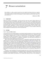
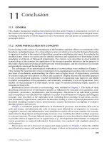
has the opposite effect on population growth rate as r. Figure 14.3 shows the general shape
of this relationship for a logistic growth model.
The phenomenological models described to this point might have to be modified if interest shifts
to smaller and smaller population sizes. Just as a population has a maximum population size (e.g., K)
it can also have a minimum population size. The population fails below this minimum number, e.g.,
the smallest number of individuals in a dispersed population needed to have a chance of sufficient
mating and reproductive success, or the minimum number of a social species needed to maintain a
viable group. This minimum population size (M)can be placed into the logistic model (Equation 14.3)
(Wilson and Bossert 1971),
dN
dt
= rN

1 −
N
K


1 −
M
N

. (14.22)
The population will go locally extinct if N falls below M.
More discussion of population loss, recovery time, and minimum population size in the context
of fishery management can be found in books by Gulland (1977) and Everhart et al. (1953), and
1
Normalized toxic “Yield” (
Y/Y
M
)
Maximum “yield”
2
1
Normalized time to recovery (T
R
/T
R(0)
)
FIGURE 14.3 The time to recover (T
R
) will increase as the “yield” or “take” due to toxicant exposure
(E
Toxicant
) increases. This modification of Figure 1.16a in Murray (1993) shows the general shape of this
relationship for a logistic growth model. The T
R(0)
is the theoretical recovery time in the absence of toxicant

exposure (T
R(0)
= 1/r) and T
R
is the recovery time at a particular yield, Y, for the steady-state population.
Yield is normalized in this figure by dividing it by the maximum possible yield (Y
M
).
© 2008 by Taylor & Francis Group, LLC
Clements: “3357_c014” — 2007/11/9 — 12:42 — page 250 — #10
250 Ecotoxicology: A Comprehensive Treatment
formulations relative to discrete growth models are provided in Murray (1993) and Haddon (2001).
Because some fisheries models based on commercial yield consider monetary costs, the applica-
tion of a common model also provides an opportunity in risk management decisions to integrate
monetary gain from fishing with monetary loss due to toxicant exposure. A management failure of
a fishery would certainly occur if, by ignoring toxicant effects, one optimized solely on the basis
of commercial fishery harvest. Perhaps the additional loss due to toxicant exposure would put the
combined consequences to the population beyond the optimal yield and the fishery would slowly
begin an inexplicable decline.
14.3 POPULATION STABILITY
Until approximately 25 years ago, the dynamics in population size described by models such as
Equations 14.3, 14.14, and 14.16 were thought to consist of an increase to some steady-state size
(e.g., K) as depicted in Figure 14.1. Deviations from this monotonic increase toward K were attrib-
uted to random processes. In 1974, Robert May published a remarkably straightforward paper in
Science demonstrating that this was not the complete story. Even the simple models described in this
chapter can display complex oscillations in population size and, at an extreme, chaotic dynamics.
Some populations do monotonically increase to a steady-state size (i.e., Stable Point in Figure 14.4).
Others tend to overshoot the carrying capacity, turn to oscillate back and forth around the carrying
capacity, andeventually settledown tothe carrying capacity (i.e., DampedOscillation in Figure 14.4).
Sizes of other populations oscillate indefinitely around the carrying capacity (i.e., Stable Cycles in

Figure 14.4). These oscillations may be between 2, 4, 8, 16, or more points. Beyond population con-
ditions resulting in stable oscillations, the number of individuals in a population at any time may be
E
D
B
A
C
4
3
2
2
1
11
1
1
1
1
2
2
2
Time
N
N
N
Time
1
2
3
4
Stable point

Damped oscillation
Stable cycle: 2 points
Stable cycle: 4 points
Chaotic
A
B
C
D
E
FIGURE 14.4 Temporal dynamics that might arise from the differential and difference models of population
growth.
© 2008 by Taylor & Francis Group, LLC
Clements: “3357_c014” — 2007/11/9 — 12:42 — page 251 — #11
Toxicants and Simple Population Models 251
best defined as chaotic (Chaotic in Figure 14.4). Population size changes in an unpredictable fashion
through time. The exact size at any time is very dependent on the initial conditions: on average,
trajectories for populations with slightly differing initial sizes separate exponentially through time
(Schaffer and Kot 1986). Although chaotic dynamics have been noted for only a few species popu-
lations (e.g., flour beetles, Tribolium castaneum (Costantino et al. 1997)), these complex population
dynamics are fostered by high r, long time lags, and periodic forcing functions like those used to
model impacts of weather extremes or insecticide spraying of target populations. There is no reason
to reject the notion that nontarget species with high rates of increase and/or significant time lags that
live near agricultural fields might exhibit chaotic dynamics.
What specific qualities determine a population’s growth dynamics? The dynamics tend to move
from stable point to damped oscillations to stable cycles to chaotic dynamics as the intrinsic rate of
increase (r), time lag (T) and/or θ increase. The rate at which population size approaches K increases
as the r increases: at a certain r, the population tends to overshoot K and move the temporal dynamics
into morecomplicated oscillations. Similarly, if the timelag (T)increases, the populationssize begins
to oscillate more and more as the population tends to overshoot and then undershoot the carrying
capacity. The exact conditions producing these different dynamics (i.e., the stability regions) have

been determined for several of the simple models described in this chapter. Table 14.1 provides those
for Equations 14.5 and 14.14 through 14.16. The derivation of these stability criteria is detailed in
May et al. (1974). May (1976a) extends the graphical approach used in Figure 14.2 to show the
conditions leading to different population dynamics.
Several points relevant to population ecotoxicology emerge from these considerations of popula-
tion dynamics. During an ecological risk assessment, the population size at a contaminated site might
be compared to that of a reference site. The observation of a smaller population at the contaminated
site relative to the uncontaminated site often leads to the conclusion of an adverse effect on the pop-
ulation. As demonstrated by the models above, some populations will characteristically have wide
variations in size through time. Others will be more stable. To compare sizes of populations from
reference and contaminated sites using data from one or a few field samplings can lead to invalid
conclusions if populations at both sites normally displayed wide oscillations. In addition, because
toxicants can affect r, T, and θ in these simple models, there is no reason to believe that toxicants will
not impact population dynamics. So, it may be important to consider pollutant effects on population
TABLE 14.1
Stability Regions for Differential (Equation 14.5) and Difference (Equations 14.15,
14.14, and 14.16) Models of Population Growth
Difference Equations
Stability Differential
Region Equation 14.5 Equation 14.15 Equation 14.14 Equation 14.16
Stable point 0 < rT < e
−1
0 < rθ<12> r > 02> r > 0
Damped oscillation e
−1
< rT < 0.5π 1 < rθ<2
Stable cycles 0.5π<rT 2 < rθ<2.69
Between 2 points 2.526 > r > 2.000 2.449 > r > 2.000
Between 4 points 2.656 > r > 2.526 2.544 > r > 2.449
Between 8 points 2.685 > r > 2.656 2.564 > r > 2.544

Between 16 or 2.692 > r > 2.685 2.570 > r > 2.564
more points
Chaotic dynamics 2.69 < rθ r > 2.692 r > 2.570
Note: Stability region information for Equations 14.5, 14.15, 14.14, and 14.16 was obtained from May (1976),
Thomas et al. (1980), May (1974), and May (1974), respectively.
© 2008 by Taylor & Francis Group, LLC
Clements: “3357_c014” — 2007/11/9 — 12:42 — page 252 — #12
252 Ecotoxicology: A Comprehensive Treatment
dynamics in addition to population size. The likelihood of a local population extinction is greatly
increased by a toxicant exposure that produces wide oscillations in addition to lowering the popula-
tion carrying capacity. The lowering of the carrying capacity brings the population numbers closer
to the minimal population number (M) and the oscillation troughs periodically bring the population
numbers even closer to M.
Higher order interactions are also possible on population dynamics. Simkiss et al. (1993)
examined the growth of blowfly (Lucilia sericata) under different combinations of food and cad-
mium. Food deprivation and cadmium concentration were additive in their effects on key growth
components (maximum larval size, development period, pupal weight, adult weight at emergence,
and fecundity). Many of these effects change r and time lags. So, the combination of cadmium
exposure and limited food availability can influence population dynamics. Nicholson (1954) had
previously shown that limited food alone produced population oscillations with Lucilia cuprina.
Simkiss et al. (1993) predicted from their studies of food and cadmium effects on blowfly pop-
ulations that “sublethal levels of cadmium might therefore lead to smaller-amplitude fluctuations
without affecting the mean population level.”
Box 14.1 Extinction Probabilities for Fruit Fly Populations under Nutritional Stress
The influence of environmental carrying capacity on the likelihood of Drosophila sp. population
extinction was quantified by Philippi et al. (1987) by manipulating the amount of food available
to cultures of different fruit fly species. In one set of experiments, food was varied from a very
restrictive 3 mL per 120 mL bottle to an excessive amount of 40 mL per 120 mL bottle. Flies
were periodically transferred to new bottles of media and the results were fit to a difference
logistic model that included Gilpin’s θ parameter:

N = N
t+1
−N
t
= rN
t
−
r
K
θ
N
(θ+1)
t
. (14.23)
The premise was that, as they had seen with species populations competing with one another
for limited resources, isolated fly populations provided with limited resources would exhibit
very widefluctuations in size. Thesefluctuations wouldincrease the chance of populationextinc-
tion. In a second set of experiments, they varied the density of flies and measured survival and
reproduction of individuals at these different densities. The resulting data were used to assess
the relative contributions of chaotic dynamics, carrying capacity reduction, and environmental
stochasticity to population persistence.
Let us assume in interpreting their results for nutritional stress that, according to
Equations 14.9, 14.18, and 14.20 and the work of Simkiss et al. (1993), toxicant exposure will
similarly impact fruit fly populations by decreasing carrying capacity. Under this assumption,
this study of food limitation has direct relevance to populations exposed to toxicants.
Much to their surprise, the food-deprived populations showed lower variability than those
with unlimited food: the stressed populations had reduced variability in their numbers. Higher
observed rates of extinction in food-deprived populations were a result of a reduced carrying
capacity and variance in growth dynamics due to environmental variability, not a shift toward
more complicated dynamics. (The stability regions for this θ-logistic model are those given for

Equation 14.15 in Table 14.1.) The environmental variability involved differences in the amount
of food placed into each bottle, the humidity, and level of bacterial contamination introduced
into cultures during handling. They conclude that the minimum viable population size (M)is
determined by deterministic and stochastic population processes but, in this case, a determin-
istic shift in population dynamics toward wider fluctuations under stressful conditions was not
responsible for the observed accelerated rates of extinction.
© 2008 by Taylor & Francis Group, LLC
Clements: “3357_c014” — 2007/11/9 — 12:42 — page 253 — #13
Toxicants and Simple Population Models 253
Sensitivity analysis for the model provided further insight into the relative importance
of changes in r and θ on the probability of population extinction. Simulations demonstrated
that extinction probabilities over a wide range of r and θ values were determined by chaotic
dynamics regardless of the level of environmental noise only if r · θ was greater than 3. At
the other extreme, systems with low r and θ values (i.e., those that we are assuming would be
characteristic of pollutant-stressed populations), recover very slowly from minor perturbations.
In this situation, extinction probability increases with environmental variability. The lowest
probabilities of extinction were in regions with 0.5 < r ·θ<2.
14.4 SPATIAL DISTRIBUTIONS OF INDIVIDUALS IN
POPULATIONS
In Section 14.2, the convenient assumption was made that a population is composed of sim-
ilar individuals occupying a spatially uniform habitat. However, individuals are often distributed
heterogeneously within a habitat that may not be homogenous itself. Some consequences of this
heterogeneity will be outlined in this section.
14.4.1 DESCRIBING DISTRIBUTIONS:CLUMPED,RANDOM,
AND UNIFORM
Individuals may be distributed uniformly, randomly, or in clusters within a habitat (Figure 14.5).
Uniform distributions are rare. Random and clumped or aggregated distributions are much more
common. The driving force for the clumping may be innate to the species (e.g., the social gather-
ing of individuals to enhance foraging or reproductive success), result from extrinsic factors (e.g.,
a landscape that is a mosaic of habitats widely differing in quality), or emerge from an interaction

of intrinsic and extrinsic factors.
Conformity of individuals within a population to these patterns can be formally tested by methods
described in various sources (i.e., Krebs 1989, Ludwig and Reynolds 1988, and Newman 1995) by
assuming that positive binomial, Poisson, and negative binomial models describe uniform, random,
Uniform
Random
Clumped
FIGURE 14.5 General distributional patterns of individuals within populations including uniform (upper
panel), random (middle panel), and clumped (lower panel) distributions.
© 2008 by Taylor & Francis Group, LLC
Clements: “3357_c014” — 2007/11/9 — 12:42 — page 254 — #14
254 Ecotoxicology: A Comprehensive Treatment
and clumped patterns, respectively. These models can also be fit to distributional data for individuals
using methods described in the cited sources.
14.4.2 METAPOPULATIONS
What arethe consequences ofan uneven distribution of individualswithin a habitat? Dothings simply
average out over the entire habitat and, as a consequence, conform to the simple population dynamics
described so far? The simple answer is no. Unique and important qualities emerge in the dynamics
and persistence ofa metapopulation. Hanski (1996) described a metapopulation as “a set of local pop-
ulations which interact via dispersing individuals among local populations; though not all local pop-
ulations in a metapopulation interact directly with every other local population.” Unique qualities of
metapopulations must be understood to appreciate the influence of toxicant exposure on populations.
14.4.2.1 Metapopulation Dynamics
Subpopulations or local populations occupy patches of the available habitat that differ slightly or
greatly relative to the ability to foster individual survival, growth, and reproduction. Consequently,
individual fitness differs among landscape patches. High quality patches may produce so many
individuals that they act as sources to other patches. Low quality patches may be so inferior that
they do not produce surplus individuals. To remain occupied, inferior sink subpopulations rely on an
influx of individuals from source patches. Some patches may be so superior relative to other marginal
patches that they are keystone habitats (O’Connor 1996) without which the metapopulation might

disappear. Which patches are sources and which are sinks may change through time depending on
factors like weather, disease, competition, orpredation pressures. In other situations in which patches
are physical islands, the source–sink structure might remain stable through time. A source–sink
dynamic emerges as essential in understanding metapopulation size and persistence on the landscape
scale (Figure 14.6).
Levins (1969, 1970; cited in Hanski (1996)) explored metapopulation dynamics with a simple
model:
dp
dt
= mp(1 −p) −ep, (14.24)
where p is the size of the metapopulation expressed as the proportion of available patches that are
occupied, e is the rate or probability of extinction in patches, and m is the rate or probability of
population reappearance in (or immigration into) vacant patches of the landscape mosaic. In more
general terms, this model states that the dp/dt is a function of the immigration and extinction rates for
patches in a habitat mosaic (Gotelli 1991). The probability of patch extinction is independent of the
regional occurrence of subpopulations (p): the likelihood of a patch being vacated is not influenced
by the proportion of nearby patches that are occupied. As we will see in the following text, this may
or may not be a good assumption. This model can be modified into a form analogous to the logistic
model for population size “with m −e being the intrinsic rate of metapopulation increase for a small
metapopulation (when p is small), while 1 −(e/m) is the equivalent of the local ‘carrying capacity,’
the stable equilibrium point toward which p moves in time” (Hanski 1996):
dp
dt
= (m −e)p

1 −
p
1 −(e/m)

. (14.25)

Gotelli (1991)provides moredetail forthis andrelated metapopulation models. He also highlights
several themes in metapopulation dynamics. First, he describes the rescue effect as a decrease in
probability of patch extinction because of the influx of individuals from nearby subpopulations, i.e.,
the assumption in Equation 14.25 is avoided that the probability of patch extinction is independent
© 2008 by Taylor & Francis Group, LLC
Clements: “3357_c014” — 2007/11/9 — 12:42 — page 255 — #15
Toxicants and Simple Population Models 255
N = 5000
Time
-
N = 5000
Local losses
and additions
of subpopulations
FIGURE 14.6 Stable metapopulation dynamics within a habitat mosaic despite periodic local extinctions.
Subpopulations vary in their ability to act as sources (size of open circles) and sinks (size of filled circle),
resulting in different probabilities of local extinction through time (upper panel). Because of the exchange
among patches, the metapopulation persists through a dynamic steady state of extinctions (− in middle panel)
and reestablishments via influx from nearby sources. New populations are also established through time via
influx from sources (+in middle panel). The net result is metapopulation persistencethrough time (lower panel).
of the regional occurrence of populations (p). The model of Hanski (described in Gotelli (1991))
includes the rescue effect by slight modification of Equations 14.24 to 14.26. In this model, the
probability of local extinction decreases as p (proportion of patches occupied) increases: emigration
from neighboring subpopulations reduces the likelihood of local extinction:
dp
dt
= mp(1 −p) −ep(1 − p). (14.26)
In Equation 14.24, the extinction rate increases as p increases. In Equation 14.26, this is true up
to a certain p. The extinction rate then begins to decline as p continues to increase.
A source of propagules such as a seed bank or dormant stage can produce a “propagule rain” that

bolsters a waning subpopulation and can influence metapopulation dynamics. In such a case, the
regional occurrence of subpopulations (p) does not impact the rate of reappearance of individuals (m)
and the rain of propagules increases the m by m(1 − p)
2
(Gotelli 1991). Under this condition and
an e that is independent of regional occurrence, a better description of metapopulation dynamics is
Equation 14.27 (Gotelli 1991),
dp
dt
= m(1 −p) −ep. (14.27)
Equation 14.28 combines the propagule rain and rescue effects:
dp
dt
= m(1 −p) −ep(1 −p). (14.28)
© 2008 by Taylor & Francis Group, LLC
Clements: “3357_c014” — 2007/11/9 — 12:42 — page 256 — #16
256 Ecotoxicology: A Comprehensive Treatment
Additional details and examples can be obtained in Lewin (1989), Gotelli (1991), Gilpin and
Hanski (1991), Pulliam and Danielson (1991), Hanski (1996), and Pulliam (1996). O’Connor (1996)
reviews metapopulation consequences of toxicant exposure.
14.4.2.2 Consequences to Exposed Populations
The paradigms of landscape ecology and metapopulation dynamics have introduced new concepts
of spatial dynamics whose implications for ecological risk assessment have only just begun to receive
attention.
(O’Connor 1996)
The metapopulation contextis quicklybeing incorporatedinto conservation biologyefforts but isonly
slowly being considered in ecotoxicology. Regardless, several consequences become obvious from
this brief sketchof metapopulationdynamics. First, a rudimentary assessmentof populationstatusin a
contaminated area requires consideration of adjacent subpopulations; otherwise, observations might
be inexplicable. Perhapstoxicity tests suggest that aspecies shouldbe absent from a contaminatedsite

but the presence of a source population produces an apparently thriving population on the site (i.e.,
the rescue effect). Second, if the lost habitat was a keystone habitat, the population consequences will
be much worse than suggested by any narrow assessment based on the percentage of total habitat lost.
Third, the creationof corridors to enhance movementamong patchescould bemore beneficialin some
cases than complete removal of contaminated media from a site. Indeed, remediation often causes
considerable disruption of habitat: a thoughtful balance of removal of polluted media from patches,
creation of corridors among patches, and building of barriers around other highly contaminated
patches could result in optimal remediation. Fourth, among migrating individuals within the mosaic
of habitats, some will have spent time in heavily contaminated patches. The result might be that
individuals exposed in one patch will have their population-level consequences manifested in a
subpopulation removed from that contaminated site. Spromberg et al. (1998) call this the effect at a
distance hypothesis because the action of a toxicant exposure occurs at a place spatially distant from
the contamination. Fifth, a sublethal effect that reduces migration-related behavior could decrease
the stability or persistence of a metapopulation by affecting the rate at which vacant habitat is refilled
from adjacent areas.
Box 14.2 Computer Projections of Metapopulation Risk in a Contaminated Habitat
Spromberg et al. (1998) developed phenomenological models for subpopulations in a habitat
with patchy distributions of individuals and toxicants. Their intent was to explore consequences
of such a metapopulation configuration and to relate the results to risk assessment activities and
possible remedial actions. They described their conceptual framework with Equations 14.24
and 14.26, and added the diffusion reaction model of Wu et al. (1993),
dN
i
dt
= N
i
f (N
i
) +


j=i
[d
ij
(N
j
−N
i
)], (14.29)
where d
ij
is the migration rate from patch i to patch j, N
i
and N
j
are the number of individuals in
patches i and j, respectively, and f () is a function of N that defines the population growth rate.
Note that, unlike previous models, the numbers of individuals in the patches is being modeled
in Equation 14.29, not the proportion of all patches that are occupied (p).
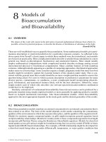
Equation 14.29 is used tosimulate the dynamicsof a metapopulationunder different contam-
ination scenarios involving three patches (Figure 14.7). Simulations included a contaminant that
© 2008 by Taylor & Francis Group, LLC
Clements: “3357_c014” — 2007/11/9 — 12:42 — page 257 — #17
Toxicants and Simple Population Models 257
quickly disappeared from a patch (e.g., a quickly degraded pesticide) and a persistent contam-
inant. The model assumed the following: (1) density-dependent growth, (2) density-dependent
patch immigration and emigration, and (3) distance-dependent movement of individuals
between patches. As an example of distance-dependent movement among patches, the dis-
tance between all three patches were similar for the model in the upper panel of Figure 14.7,
but the distance between the two outer patches in the model at the bottom of this figure was
twice as far as the distance from any one of these outer patches to the center patch. For the

model in the lower panel, the distance-dependent movement between an outer patch and the
central one was much higher than the movement between the two outside patches. Computation
of migration rate from patch i to j was done with the simple equation, d
ij
= (N
i
H
j
)/D
ij
, where
H
j
is the habitat available to be occupied in patch j, and D
ij
is the distance between the two
patches.
Other model assumptions included a constant carrying capacity and minimum popula-
tion size for a patch, no avoidance of contaminated habitat, no compensatory reproduction
due to the presence of toxicant, a Poisson distribution to define the probability of an indi-
vidual being exposed to a toxicant in the contaminated patch, constant bioavailability of
toxicant, and the occurrence of no other stochastic disturbances (e.g., no weather-related
mortalities).
The results of the simulations are easily summarized. A toxic effect can be seen in sub-
populations of nearby, uncontaminated patches due to the movement of individuals into those
patches from a contaminated patch. Again, the authors refer to this as the hypothesis of effect
at distance. Toxicant-induced reduction in subpopulation size in one patch results in a higher
rate of movement of individuals into that patch. In the model in the lower panel of Figure 14.7,
even 100% mortality in the contaminated patch does not produce a local extinction. Individu-
als move into the vacated patch from the other patches. One noteworthy conclusion derived

from the simulations was that a reference population picked from near a contaminated site
might not produce useful information in an ecological risk assessment. Although not contam-
inated, the subpopulation occupying that clean patch may still be impacted by the toxicant
due to migration of individuals from the contaminated patch. Conversely, remediation of a
site can result in improvements in population viability in patches outside that containing the
toxicant.
d
13
d
31
d
31
d
32
d
23
d
12
d
21
3
1
2
d
13
d
32
d
23
d

12
3
2
1
d
21
FIGURE 14.7 The three patch metapopulations
simulated by Spromberg et al. (1998). Patches with
skull and cross bones indicate contaminated patches
and the open symbol represents uncontaminated
patches. As described in the text, d
ij
indicates the
migration rate from patch i to patch j. (Modified
from Figure 1 of Spromberg et al. (1998).)
© 2008 by Taylor & Francis Group, LLC
Clements: “3357_c014” — 2007/11/9 — 12:42 — page 258 — #18
258 Ecotoxicology: A Comprehensive Treatment
14.5 SUMMARY
Population-based assessment endpoints are beginning to occupy a more prominent role in ecological
risk assessments. To accelerate this change, relevant concepts and methods need to be described so
that ecotoxicologists feel comfortable with their application. Population-based metrics of effect will
need to accumulatein databases such as theAQUIRE database maintained by the U.S. Environmental
Protection Agency. Obviously, consilience among levels is essential as the new, population-centered
paradigm emerges. Linkage to individual-basedeffects can bemade withindividual-based population
models such as some of the demographic analyses described in the next chapter. However, data must
be collected so that these links can be made. Presently, they often are not collected in an appropriate
manner. Linkage to community-level effects is also possible with the context developed in this
chapter. For example, the metapopulation formulations (e.g., Equation 14.25) are closely related
to the community succession models (MacArthur–Wilson model) used by Cairns et al. (1986) to

predict toxicant effects to protozoan community processes.
14.5.1 SUMMARY OF FOUNDATION CONCEPTS AND PARADIGMS
• A population-based paradigm for assessing ecological risk is slowly beginning to
share importance with the currently dominant paradigm based on metrics for effect to
individuals.
• Phenomenological models of population dynamics provide an understanding of possible
behaviors of populations, including those experiencing toxicant exposure.
• Toxicant exposure can change the population qualitiesreflected in themodel parameters, r,
λ, K, T, g, T
R
, M, and θ.
• Effects of toxicant exposure can be included in conventional growth models as a density-
independent population loss.
• Toxicant exposure can reduce population size.
• Toxicant exposures can change population dynamics.
• Toxicant exposure can result in an increased probability of population extinction.
• Population sustainability and recovery with toxicant exposure can be modeled with modi-
fications to methods used to manage harvested, renewable resources such as a commercial
or recreational fishery.
• Increased toxicant exposure may not necessarily result in a decrease in population produc-
tion rate. Populations can loose a number of their surplus offspring without a significant
change in population viability. On either side of the maximum sustainable loss to tox-
icant exposure (“yield”) are equal points of excess production by the population (see
Section 14.2.4).
• Expression of loss due to toxicant exposure in terms used by managers of renewable
resources, for example, commercial fishery managers, allows the integration of toxicant
and fishing/harvesting activities in assessments of resource sustainability.
• Temporal dynamics of populations can take several forms including monotonic increase
to carrying capacity, damped oscillations to carrying capacity, stable oscillations about
carrying capacity, or chaotic dynamics. These dynamics are determined by combinations

of r, T, and θ (see Table 14.1). Because r, T, and θ can be changed by toxicant exposure,
population dynamics can be changed by toxicant exposure.
• Individuals can benonrandomly distributedin available habitat. Distributionof individuals
in a population can be influenced by innate qualities of the species and/or qualities of the
environment, including the presence of toxicants.
• Metapopulation dynamics influence the probability of population extinction in landscape
mosaics contaminated with toxicants.
© 2008 by Taylor & Francis Group, LLC
Clements: “3357_c014” — 2007/11/9 — 12:42 — page 259 — #19
Toxicants and Simple Population Models 259
• Habitats have finite, but fluctuating, capacities to support a species population and tox-
icants can lower (e.g., reduction of amount of food or suitable habitat) or increase (e.g.,
remove a competitor or predator) the carrying capacity of a habitat.
• Assessment of toxicant exposure consequences to a metapopulation must consider source–
sink dynamics, keystone habitats, and the possibilities of the rescue effect and a significant
propagule rain effect.
• Creation of corridors between patches or isolation of the contaminated patch may greatly
influence metapopulation viability. These actions should be considered in addition to
conventional removal of contaminated media in remediation plans.
REFERENCES
Barnthouse, L.W., Suter, G.W., II, Rosen, A.E., and Beauchamp, J.J., Estimating responses of fish populations
to toxic contaminants, Environ. Toxicol. Chem., 6, 811–824, 1987.
Birch, L.C., The intrinsic rate of natural increase of an insect population, J. Anim. Ecol., 17, 15–26,
1948.
Braithwaite, R.B., The structure of a scientific system, In The Concept of Evidence, Achinstein, P. (ed.), Oxford
University Press, Oxford, UK, 1983, pp. 44–62.
Cairns, J., Jr., Pratt, J.R., Niederlehner, B.R., and McCormick, P.V., A simple cost-effective multispecies
toxicity test using organisms with a cosmopolitan distribution, Environ. Monit. Assess., 6, 207–220,
1986.
Caswell, H., Demography meets ecotoxicology: Untangling the population level effects of toxic substances,

In Ecotoxicology. A Hierarchical Treatment, Newman, M.C. and Jagoe, C.H. (eds.), CRC Press/Lewis
Publishers, Boca Raton, FL, 1996, pp. 255–292.
Costantino, R.F., Desharnais, R.A., Cushing, J.M., and Dennis, B., Chaotic dynamics in an insect population,
Science, 275, 389–391, 1997.
Daniels, R.E. and Allan, J.D., Life table evaluation of chronic exposure to a pesticide, Can. J. Fish. Aquat. Sci.,
38, 485–494, 1981.
DeAngelis, D.L. and Gross, L.J. (eds.), Individual-based Models and Approaches in Ecology, Chapman & Hall,
New York, 1992.
Emlen, J.M., Terrestrial population models for ecological risk assessment: A state-of-the-art review, Environ.
Toxicol. Chem., 8, 831–842, 1989.
EPA, Summary Report on Issues in Ecological Risk Assessment, EPA/625/3-91/018 February 1991, NTIS,
Springfield, 1991.
Everhart, W.H., Eipper, A.W., and Youngs, W.D., Principles of Fishery Science, Cornell University Press,
Ithaca, NY, 1953.
Forbes, V.E. and Calow, P., Is the per capita rate of increase a good measure of population-level effects in
ecotoxicology? Environ. Toxicol. Chem., 18, 1544–1556, 1999.
Gard, T.C., A stochastic model for the effects of toxicants on populations, Ecol. Modell., 51, 273–280,
1990.
Gard, T.C., Stochastic models for toxicant-stressed populations, Bull. Math. Biol., 54, 827–837, 1992.
Gilpin, M.E. and Ayala, F.J., Global models of growth and competition, Proc. Natl. Acad. Sci. USA, 70,
3590–3593, 1973.
Gilpin, M.E. and Hanski, I. (eds.), Metapopulation Dynamics: Empirical and Theoretical Investigations,
Harcourt Brace Jovanovich, London, UK, 1991.
Gotelli, N.J., Metapopulation models: The rescue effect, the propagule rain, and the core-satellite hypothesis,
Am. Nat., 138, 768–776, 1991.
Gulland, J.A., Fish Population Dynamics, John Wiley & Sons, London, UK, 1977.
Haddon, M., Modelling and Quantitative Methods in Fisheries, Chapman and Hall/CRC Press, Boca Raton,
FL, 2001.
Hanski, I., Metapopulation ecology, In Population Dynamics in Ecological Space and Time,
Rhodes, O.E., Jr., Chesser, R.K., and Smith, M.H. (eds.), University of Chicago Press, Chicago,

IL, 1996, pp. 13–43.
© 2008 by Taylor & Francis Group, LLC
Clements: “3357_c014” — 2007/11/9 — 12:42 — page 260 — #20
260 Ecotoxicology: A Comprehensive Treatment
Krebs, C.J., Ecological Methodology, Harper Collins Publishers, Inc., New York, 1989.
Kuhn, T.S., The Structure of Scientific Revolutions, University of Chicago Press, Chicago, IL, 1962.
Lakatos, I., Falsification and the methodology of scientific research programmes, In Criticism and the Growth of
Knowledge, Lakatos, I. and Musgrave, A. (eds.), Cambridge University Press, Cambridge, UK, 1970,
pp. 91–196.
Levins, R., Some demographic and genetic consequences of environmental heterogeneity for biological control,
Bull. Entomol. Soc. Am., 15, 237–240, 1969.
Levins, R., Extinction, Lect. Math. Life Sci., 2, 75–107, 1970.
Lewin, R., Sources and sinks complicate ecology, Science, 243, 477–478, 1989.
Ludwig, J.A. and Reynolds, J.F., Statistical Ecology. A Primer on Methods and Computing, John Wiley & Sons,
New York, 1988.
May, R.M., Biological populations with nonoverlapping generations: Stable points, stable cycles, and chaos,
Science, 186, 645–647, 1974.
May, R.M., Theoretical Ecology. Principles and Applications, W.B. Saunders Co., Philadelphia, PA, 1976a.
May, R.M., Simple mathematical models with very complicated dynamics, Nature, 261, 459–467, 1976b.
May, R.M., Conway, G.R., Hassell, M.P., and Southwood, T.R.E., Time delays, density-dependence and
single-species oscillations, J. Anim. Ecol., 43, 747–770, 1974.
May, R.M. and Oster, G.F., Bifurcation and dynamic complexity in simple ecological models, Am. Nat., 110,
573–599, 1976.
Moriarty, F., Ecotoxicology. The Study of Pollutants in Ecosystems, Academic Press, Inc., London, UK,
1983.
Murray, J.D., Mathematical Biology, Springer-Verlag, Berlin, 1993.
Newman, M.C., Quantitative Methods in Aquatic Ecotoxicology, CRC Press/Lewis Publishers, Boca Raton,
FL, 1995.
Newman, M.C., Fundamentals of Ecotoxicology, CRC Press/Lewis Publishers, Boca Raton, FL, 1998.
Newman, M.C. and Jagoe, R.H., Allozymes reflect the population-level effect of mercury: Simulations of the

mosquitofish (Gambusia holbrooki Girard) GPI-2 response, Ecotoxiology, 7, 141–150, 1998.
Nicholson, A.J., An outline of the dynamics of animal populations, Aust. J. Zool., 2, 9–65, 1954.
Norton, S.B., Rodier, D.J., Gentile, J.H., Van der Schalie, W.H., Wood, W.P., and Slimak, M.W.,
A framework for ecological risk assessment at the EPA, Environ. Toxicol. Chem., 11, 1663–1672,
1992.
O’Connor, R.J., Toward the incorporation of spatiotemporal dynamics into ecotoxicology, In Population
Dynamics in Ecological Space and Time. Rhodes, O.E., Jr., Chesser, R.K. and Smith, M.H. (eds.),
University of Chicago Press, Chicago, IL, 1996, pp. 281–317.
Philippi, T.E., Carpenter, M.P., Case, T.J., and Gilpin, M.E., Drosophila population dynamics: Chaos and
extinction, Ecology, 68, 154–159, 1987.
Popper, K.R., Objective Knowledge. An Evolutionary Approach, Clarendon Press, Oxford, UK, 1972.
Pulliam, H.R., Sources and sinks: Empirical evidence and population consequences, In Population Dynamics
in Ecological Space and Time, Rhodes, O.E., Jr., Chesser, R.K., and Smith, M.H. (eds.), University of
Chicago Press, Chicago, IL, 1996, pp. 45–69.
Pulliam, H.R. and Danielson, B.J., Sources, sinks, and habitat selection: Alandscape perspective on population
dynamics, Am. Nat., 137, S50–S66, 1991.
Schaffer, W.M. and Kot, M., Chaos in ecological systems: The coals that Newcastle forgot. TREE, 1, 58–63,
1986.
Sibly, R.M., Effects of pollutants on individual life histories and population growth rates, In Ecotoxicology.
A Hierarchical Treatment, Newman, M.C. and Jagoe, C.H. (eds.), CRC Press/Lewis Publishers, Boca
Raton, FL, 1996, pp. 197–223.
Simkiss, K., Daniels, S., and Smith, R.H., Effects of population density and cadmium toxicity on growth and
survival of blowflies, Environ. Pollut., 81, 41–45, 1993.
Spromberg, J.A., John, B.M., and Mandis, W.G., Metapopulation dynamics: Indirect effects and multiple
distinct outcomes in ecological risk assessment, Environ. Toxicol. Chem., 17, 1640–1649, 1998.
Thomas, W.R., Pomerantz, M.J., and Gilpin, M.E., Chaos, asymmetricgrowthand group selection fordynamical
stability, Ecology, 6, 1312–1320, 1980.
Verhulst, P.F., Notice sur la loi que la population suit dans son accroissement, Corr. Math. et Phys., 10, 113–121,
1838.
© 2008 by Taylor & Francis Group, LLC

Clements: “3357_c014” — 2007/11/9 — 12:42 — page 261 — #21
Toxicants and Simple Population Models 261
Waller, W.T., Dahlberg, M.L., Sparks, R.E., and Cairns, J., Jr., A computer simulation of the effects of super-
imposed mortality due to pollutants of fathead minnows (Pimephales promelas), J. Fish. Res. Board
Can., 28, 1107–1112, 1971.
Wilson, E.O. and Bossert, W.H., A Primer of Population Biology, Sinauer Associates, Inc., Sunderland, MA,
1971.
Wu, J., Vankat, J.L., and Barlas, Y., Effects of patch connectivity and arrangement on animal metapopulation
dynamics: A simulation study, Ecol. Modell., 65, 221–254, 1993.
© 2008 by Taylor & Francis Group, LLC