ECOTOXICOLOGY: A Comprehensive Treatment - Chapter 15 pot

Clements: “3357_c015” — 2007/11/9 — 18:21 — page 263 — #1
15
Toxicants and Population
Demographics
There’s a special providence in the fall of a sparrow. If it be now, ’tis not to come if it be not to come,
it will be now; if it be not now, yet it will come: the readiness is all
(Hamlet Act V, SC II)
15.1 DEMOGRAPHY: ADDING INDIVIDUAL
HETEROGENEITY TO POPULATION MODELS
Discussion so far grew from phenomenological models involving identical and uniformly distrib-
uted individuals to metapopulation models incorporating spatial heterogeneity. Now, demography,
the quantitative study of death, birth, age, migration, and sex in populations, will be explored. Dif-
ferences among individuals produce distinct vital rates, that is, rates of death, birth, transition to the
next life stage, and migration. Combined, vital rates determine a population’s overall characteristics.
In fact, population vital rates were aggregated earlier into summary statistics such as the intrinsic
rate of increase, resulting in hidden information and incomplete insight. Finally, metapopulation
models including demographic vital rates can be discussed briefly to get the fullest description of
and most realistic predictions of population consequences of toxicant exposure. Variation in vital
rates can be added also to render a stochastic model. Such a model could be applied to estimate
the probability of local extinction for a metapopulation based on contaminant-induced changes in
vital rates.
Demographic analysis allows thequalities and fate of toxicant-exposed populations to be determ-
ined. In the recent past, conventional ecotoxicological precepts suggested that a species population
will remain viable if the most sensitive life stage of the species is “protected,” e.g., toxicant con-
centrations do not exceed the no observed effect level (NOEC) or MATC concentration for that
life stage. Early life stage testing results were applied under the premise that the population will
remain viable if the weakest link in an individual’s various life stages was protected. But this is
not always true. Newman (1998) refers to this false paradigm as the weakest link incongruity. The
most sensitive stage of an individual’s life cycle might not be the most crucial relative to population
vitality or viability (Kammenga et al. 1996, Petersen and Petersen 1988). This will become obvious
as we discuss reproductive value, elasticity, and related topics below. Fortunately, ecotoxicology is

rapidly moving toward a more balanced inclusion of demographic analysis (e.g., Bechmann 1994,
Chaumot et al. 2003, Daniels and Allan 1981, Koivisto and Ketola 1995, Martinez-Jerónimo et al.
1993, Münzinger and Guarducci 1988, Pesch et al. 1991, Spurgeon et al. 2003). Required now
is a sustained and insightful integration of demography into assessments of ecological risk. The
intent of this chapter is to contribute to this integration by describing foundation demographic con-
cepts and methods. Straightforward algebraic (e.g., Marshall 1962) and matrix (e.g., Caswell 1996,
Lefkovitch 1965, Leslie 1945, 1948) formulations will be described because both are applied in
population ecotoxicology.
15.1.1 S
TRUCTURED POPULATIONS
Age-, stage-, and sex-dependent vital rates will be considered in this section. Age data may be
applied when available or, alternatively, analyses might focus on vital rates at different life stages
263
© 2008 by Taylor & Francis Group, LLC
Clements: “3357_c015” — 2007/11/9 — 18:21 — page 264 — #2
264 Ecotoxicology: A Comprehensive Treatment
such as larval →juvenile →and adult stages. For example, the effects of dioxin and polychlorinated
biphenyls (PCBs) on Fundulus heteroclitus populations were modeled by considering the following
life stages: embryos →larvae →28-day larvae →1-year-old adults →2-year-old adults →3-year-
old adults (Munns et al. 1997). Sex-dependent vital rates can be important too but our focus here
will remain primarily on females of differing ages or stages.
15.1.2 BASIC LIFE TABLES
Life tables or schedules are constructed either for mortality alone, both mortality and birth (natality),
or mortality, natality, and migration combined. Obviously, analysis of a metapopulation requires the
inclusion of movement among subpopulations. In this chapter, we will only show calculations that
are relevantto populationswith no migration; however, inclusion of these methods in metapopulation
models would be possible using concepts described in the last chapter.
Data for life tables are gathered in three ways. To produce a cohort life table, a cohort of
individuals is followed through time with tabulation of mortality alone, or mortality and natality.
As an example, a group of 1000 young-of-the-year (YOY0+) may be tagged during the calving

season and survival of these calves followed through the years of their lives. Other cohorts present
in the population are ignored. In contrast, a horizontal life table includes measurements about all
individuals in the population at a particular time and several cohorts are included. All individuals
within the various age classes are counted and the associated data summarized in a horizontal table.
An important point to note here is that the results of cohort and horizontal life tables will not always
be identical for the same population. They would be identical only if environmental conditions were
sufficiently stable so that vital rates remain fairly independent of time, that is, independent of the
specific cohort(s) from which they were derived. In a composite life table, data are collected for
several cohorts and combined. For example, a team of game managers might tag newborns during
four consecutive calving seasons, follow the four cohorts through time, and then combine the final
results in one table.
15.1.2.1 Survival Schedules
Oh, Death, why canst thou sometimes be timely?
(Melville, Moby Dick 1851)
Sometimes life schedules quantify death only. Life insurance companies or some ecological risk
assessors might correctly pay most attention to the likelihood of dying and consider natality as
irrelevant. The associated tabulations are called l
x
schedules because, by convention, the symbol l
x
designates the number or proportion of survivors in the age class, x. Often, l
x
is expressed as a
proportion of the original number of newborns surviving to age x. In that form, it also estimates the
probability of survival to age x.
From l
x
schedules, simple estimates are made of the number of deaths (d
x
= l

x
− l
x+1
), rate
of mortality (q
x
), and expected lifetime for an individual surviving to age x (e
x
). Like l
x
,ifd
x
is
expressed as a proportion dying instead of actual number dying, d
x
estimates the probability of dying
in the interval x to x +1. These estimates may be expressed as a simple quotient (e.g., q
x
= d
x
/l
x
)or
normalized to a specific number of individuals in the age class such as deaths per 1000 individuals
(e.g., 1000q
x
= 1000(d
x
/l
x

)) (Deevey 1947).
The mean expected length of life beyond age x for an individual who survived to age x (e
x
) can
be estimated for any age class (x) by dividing the area under the survival curve after x by the number
of individuals surviving to age x (Deevey 1947),
e
x
=

∞
x
l
x
dx
l
x
. (15.1)
© 2008 by Taylor & Francis Group, LLC
Clements: “3357_c015” — 2007/11/9 — 18:21 — page 265 — #3
Toxicants and Population Demographics 265
With a basic l
x
table, the e
x
in the above equation can be approximated with the l
x
and L
x
(number

of living individuals between x and x +1 in age):
L
x
=

x+1
x
l
x
dx. (15.2)
A simple linear approximation of L
x
in the above equation is L
x
= (l
x
+ l
x+1
)/2. Obviously,
the ∞in the summations here and elsewhere become the age at the bottommost row of the completed
life table. These L
x
approximations are summed in the life table from the bottommost row up to and
including the age of interest (x). The e
x
value for an age class is then estimated by dividing this sum
(T
x
)byl
x

(i.e., e
x
= T
x
/l
x
). (The T
x
is the total years lived by all individuals in the x age class.)
The e
0
or expected life span for an individual at the beginning of the life table (i.e., a neonate),
and its associated variance are estimated by Leslie et al. (1955) and described in detail by
Krebs (1989).
A quick check of Section 13.1.3.1, Accelerated Failure Time and Proportional Hazard Models,
will show a striking similarity between those epidemiological methods for modeling mortality and
these simple life table methods. In fact, the method just described is simply one method for sum-
marizing survival information. Methods, models, and hypothesis tests described in Section 13.1.3.1
or 9.2.3 can be, and often are, applied in demography. As an example, Spurgeon et al. (2003) applied
a Weibull model to survival data for metal-exposed earthworms.
Box 15.1 Death, Decline, and Gamma Rays
As the possibility of nuclear war emerged in the 1950s and 1960s, researchers began to explore
the ecological effects of intense irradiation. Ecological entities from individuals (e.g., Casarett
1968) to populations (e.g., Marshall 1962) to entire ecosystems (e.g., Woodwell 1962, 1963)
were irradiated in numerous studies to determine the consequences. One study placed cultures
of Daphnia pulex (50 individuals per culture) at a series of distances from a 5000 Curie cobalt
(
60
Co) source. The Daphnia experienced continuous gamma irradiation at dose rates of 0, 22.8,
47.9, 52.2, 67.5, and 75.9 R/h. Survival was monitored for35 days andlife schedules constructed

for each irradiated population (Table 15.1). Instead of estimating a simple LD50 at a set time,
Marshall (1962) used demographic methods to summarize the population consequences of
irradiation. This allowed estimation of the change in average life expectancy as a consequence
TABLE 15.1
Survival Rates (l
x
as a Proportion of the Ori-
ginal Population) for Daphnia pulex Continuously
Irradiated with Radiocobalt
Dose Rate (R/h)
Days (x) 0 22.8 47.9 52.2 67.5 75.9
0 1.00 1.00 1.00 1.00 1.00 1.00
7 0.98 0.98 0.98 0.98 0.98 0.96
14 0.98 0.96 0.98 0.94 0.96 0.94
21 0.98 0.88 0.48 0.16 0.12 0.02
28 0.19 0.53 0.00 0.00 0.00 0.00
35 0.00 0.00 0.00 0.00 0.00 0.00
Source: Modified from Table I in Marshall (1962).
© 2008 by Taylor & Francis Group, LLC
Clements: “3357_c015” — 2007/11/9 — 18:21 — page 266 — #4
266 Ecotoxicology: A Comprehensive Treatment
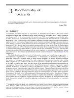
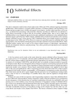
FIGURE 15.1 Calculated life expectancies for
three age classes of Daphnia pulex as a function
of gamma irradiation dose rate.
Dose rate
(
roent
g
ens/h
)

0 22.8 47.9 52.2 67.5 75.9
Average life expectancy (days)
0
1
2
3
0–7 day
7–14 day
14–21 day
of dose rate (Figure 15.1). For the sake of brevity, calculations were done here by using weekly
age classes, not daily age classes as done in the original publication. Even with this simplified
analysis, the decrease in average life expectancy for the different age classes was obvious. Note
that in Figure 15.1 there is a suggestion of a hormetic effect at 22.8 R/h (see Sections 9.1.4
and 16.2 for more discussion of hormesis).
Obviously, survivalfunctions and lifeexpectancies provide valuable insights intopopulation
consequences and, when combined later with natality data (Box 15.2), of population fate under
different intensities of irradiation.
15.1.2.2 Mortality–Natality Tables
There is an appointed time for everything, and a time for every affair under the heavens. A time to be
born, a time to die
(Ecclesiastes 3)
The inclusion of information on births (natality, m
x
) in addition to mortality (l
x
) allows expansion of
this approach. The resulting schedules are called l
x
m
x

tables. Often, l
x
m
x
tables quantify information
for females alone because the reproductive contribution of males to the next generation is much more
difficult to estimate than that of females. An m
x
is estimated for females as the average number of
female offspring produced per female of age x. Several useful population qualities can be estimated
after the age-specific birth rates (m
x
) and l
x
values are known. The expected number of female
offspring produced in the lifetime of a female or net reproductive rate (R
0
) is defined by the following
equation (Birch 1948):
R
0
=

∞
0
l
x
m
x
dx. (15.3)

This ratio of female births in two successive generations is estimated as the sum of the products
l
x
m
x
for all age classes: R
0
= l
x
m
x
. Knowing R
0
, a mean generation time (T
c
) can be calculated
by dividing the sum of all the xl
x
m
x
values by R
0
. (The midpoint of interval x to x +1 is used as “x”
in generating the product, xl
x
m
x
. For example, (0 +1)/2 or 0.5 would be used for x of the interval 0
© 2008 by Taylor & Francis Group, LLC
Clements: “3357_c015” — 2007/11/9 — 18:21 — page 267 — #5

Toxicants and Population Demographics 267
to 1-year-old.) It can also be estimated with the following equation; however, an estimate of the
intrinsic rate of increase (r) would be needed:
T
c
=
ln R
0
r
. (15.4)
The intrinsic rate of increase (r) could be grossly estimated with Equation 15.5, which is a simple
rearrangement of Equation 15.4:
r =
ln R
0
T
c
. (15.5)
This rough estimate of r can then be used as an initial estimate in the Euler–Lotka equation
(Equation 15.6) (Euler 1760, Lotka 1907), whichbecomes Equation 15.7 for theapproximate method
applied to simple life tables (Birch 1948):

∞
0
e
−rx
l
x
m
x

dx = 1, (15.6)
ω

x=0
l
x
m
x
e
−rx
= 1, (15.7)
where ω indicates the result for the bottommost row of the life table. The x, l
x
, and m
x
values, and
the initial estimate of r from Equation 15.5 are placed into Equation 15.7, and the equation solved.
Next, the value of r is changed slightly and the equation is solved again. This process is repeated with
different estimates of r until an r is found for which the equality is “close enough.” This final value
of r is the best estimate from the life table. The assumptions here are that the population is increasing
exponentially and the population is stable; however, Stearns (1992) states that this approach is robust
to violations of the assumption of a stable age structure.
Astablepopulation is one in which the distribution of individualsamong thevarious age (or stage)
classes remains constant through time. The structure of such a population is called its stable age
structure. Any population with a constant r or λ will eventually take on a stable age structure: the
eventual distribution of individuals among the age classes will be a consequence of age-specific
birth and death rates. The proportion of all individuals in age class x for a stable population (C
x
)
is defined by Equation 15.8 (see Birch (1948), Caswell (1996), Newman (1995), or Stearns (1992)

for more details):
C
x
=
λ
−x
l
x

ω
i=0
λ
−i
l
i
. (15.8)
Remember from the last chapter that λ = e
r
.
Reproductive value (V
A
) is a measure of the number of females that will be produced by a female
of age A under the assumption of a stationary population. A stationary population is one in which
simple replacement is occurring (i.e., R
0
= 1orr = 0). Therefore, by definition, neonates will have
a V
A
(=V
0

) of 1 because each will just replace herself in a stationary population. Postreproductive
females will have V
A
values of 0. It follows that the V
A
can be envisioned as the reproductive value for
a specific class, x, divided by that of a neonate (i.e., V
A
= V
x
/V
0
).
Age- or stage-specific reproductive values for a population are a valuable set of measures of the
contribution of offspring to be expected from each age class to the next generation. The relative
sizes of V
A
values for the different age classes suggest the value of each age class in contribut-
ing new individuals to the next generation. It takes simultaneously into account the facts that a
© 2008 by Taylor & Francis Group, LLC
Clements: “3357_c015” — 2007/11/9 — 18:21 — page 268 — #6
268 Ecotoxicology: A Comprehensive Treatment
female has survived to age x and that she has an age-specific capacity to produce young. (See Ste-
arns (1992) or Wilson and Bossert (1971) for a detailed description of V
A
and stepwise derivation
of equations associated with V
A
. Newman (1995) provides a detailed example of applying V
A

to
ecotoxicology.)
V
A
=
ω

x=A
l
x
l
A
m
x
. (15.9)
Goodman (1982) (detailed in Stearns 1992) provides Equation 15.10, a modification of the
Euler–Lotkaequation, to describeV
A
in anexponentially growing population. Thelower contribution
of offspring born later relative to the contribution of those born earlier is included in this equation
(Stearns 1992, Wilson and Bossert 1971),
V
A
=
e
r(A−1)
l
A
ω


x=A
e
−rx
l
x
m
x
. (15.10)
This demographic metric provides valuable insights relevant to the weakest link incongruity.
The reproductive value (V
A
) suggests the loss of individuals that would otherwise come into the
next generation if one individual of a certain age class were removed from the population. The
most valuable individuals in this context are not always the young stages that are most sensitive to
toxicant action. In general, one could argue that individuals just entering their reproductive stage
might be more valuable as they usually have very high reproductive values (Wilson and Bossert
1971). Regardless, conventional generalizations are insufficient that protection of the most sensitive
stage based on life stage testing will ensure a viable population. This point will be reinforced later
in discussions of sensitivity and elasticity. A demographic analysis should be done in order to make
any judgments about the population consequences of toxicant exposure.
There is also a definite linkage between this demographic concept of reproductive value and those
described earlier for sustainable harvest. Owing to aggregation of information, stimulation of harvest
based solely on total numbers would be less effective than estimation based on a fuller knowledge
of age- or size-specific harvests and reproductive values. Stock assessment models including size-
specific harvesting gear have direct relevance to age-specific mortality in populations due to toxicant
exposure.
Box 15.2 Death, Decline, Gamma Rays, and Birth
Marshall (1962) measured natality in addition to mortality for D. pulex exposed to gamma
radiation. Let us add these natality data (Table 15.2) to that already analyzed for mortality
(Table 15.1). Again, data are pooled here into weekly age classes.

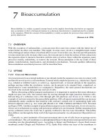
The Euler–Lotka equation (Equation 15.7) was used to estimate the intrinsic rates
of increase for the irradiated populations (Figure 15.2). Notice the general decrease in
r until it drops below 0 at approximately 67.5 R/h. At that point, the population would
slowly drop in size until extinction occurred. The stable population structures (Figure 15.3)
show a trend from a control population with many young to highly dosed populations
with proportionally fewer young and many more old individuals. Given this shift, it is
interesting to note that Aubone (2004) found decreased population stability with fishery
practices that skewed the stable age structure toward juveniles. From the lowest to the highest
dose, the generation times dropped rapidly from 13.6 to only 4.8–6.0 days.
© 2008 by Taylor & Francis Group, LLC
Clements: “3357_c015” — 2007/11/9 — 18:21 — page 269 — #7
Toxicants and Population Demographics 269
TABLE 15.2
Natality (m
x
) for D. pulex Continuously Irradiated with
Radiocobalt
Dose Rate (R/h)
Day (x to x + 1) 0 22.8 47.9 52.2 67.5 75.9
1–6 2.63 2.29 1.94 1.88 0.94 0.39
7–13 14.64 10.84 1.60 0.45 0.18 0.22
14–20 3.29 1.06 0.02
21–27 0.35
28–35 0.31
Source: Modified from Table II in Marshall (1962).
Dose rate (roentgens/h)
0 22.8 47.9 52.2 67.5 75.9
Intrinsic rate of increase (
r )
0.3

0.2
0.1
0.0
−0.1
FIGURE 15.2 Drop in intrinsic rate of
increase (r) with dose rate for D. pulex
cultures.
Age class (day)
0–7
7–14
14–21 21–28
28–35
Stable proportion
2
1
0 roentgens/h
22.8 roentgens/h
47.9 roentgens/h
52.2 roentgens/h
67.5 roentgens/h
75.9 roentgens/h
FIGURE 15.3 Shift in stable population
structure for D. pulex cultures exposed to
different dose rates of gamma radiation.
© 2008 by Taylor & Francis Group, LLC
Clements: “3357_c015” — 2007/11/9 — 18:21 — page 270 — #8
270 Ecotoxicology: A Comprehensive Treatment
Clearly, meaningful information relative to population changes and consequences were
obtained from this simple demographic analysis. Irradiation reduced average life expectancy
and generation time. Population growth rate decreased with dose until it fell below simple

replacement at approximately 67.5 R/h. Populations receiving such doses would disappear
after a few generations. The age structure of the populations shifted to a preponderance of older
individuals. In our opinion, these insights are much more meaningful than those provided by
LD50 and NOEC data.
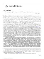
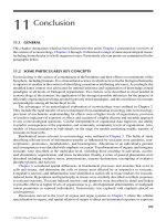
15.2 MATRIX FORMS OF DEMOGRAPHIC MODELS
To this point, discussion was simplified by avoiding matrix algebra. However, the approach
becomes much more effective with matrix formulations for demographic qualities (Figure 15.4).
Matrix formulations have existed for some time: Leslie (1945, 1948) articulated the founda-
tion matrix approach to age-structured demographics. To begin, the rudimentary matrix oper-
ations needed to apply a matrix approach will be described in the next section. Much, but
not all, of the description of basic matrix mathematics comes directly from Chapter 1 of
Emlen (1984).
15.2.1 BASICS OF MATRIX CALCULATIONS
A matrix is simply a rectangular array of numbers or variables. Its size is usually designated by
the number of rows (i) and columns (j), for example, a 4 × 1or4× 4 matrix. A matrix com-
posed of only one row is called a vector. A 1 × 1 matrix is a scalar, e.g., the number, 12, is a
scalar:




2
5
6
3




= 4 × 1 matrix = a,





12517 3
2301210
555 3
12713 5




= 4 × 4 matrix = A.
Matrices are conventionally designated with boldfaced, capital letters (e.g., A), except vectors
that are designated as boldface, small letters (e.g., a above). Scalars are written as small letters
without boldfacing. A matrix can be designated generally as A ={a
ij
} where i is row position and
j is column position. For example, element a
13
in A is 17.
Wewill need to do simple matrix multiplication in thedemographic models that follow; therefore,
a quickreview of matrix multiplication is presented here. Multiplicationof ascalar bya matrix (b×A)
Age-structured model
Stage-structured model
0
1
2
3
0

1
2
3
F
3
F
2
F
1
F
3
F
2
F
1
P
2
P
1
P
0
P
2
P
3
P
1
P
0
G

0
G
1
G
2
FIGURE 15.4 An illustration of age- and stage-structured population models. The age-structured model
specifies natality (F) and probability of moving to the next age class (P). The stage-structured model specifies
the natality (F), probability of moving to the next stage class (G), and probability of remaining in the stage
class (P).
© 2008 by Taylor & Francis Group, LLC
Clements: “3357_c015” — 2007/11/9 — 18:21 — page 271 — #9
Toxicants and Population Demographics 271
is very straightforward. Each individual element of the matrix is simply multiplied by the scalar.
Let b be a scalar with value 12 and A bea2×2 matrix:
12 ×A = 12

a
11
a
12
a
21
a
22

=

12a
11
12a

12
12a
21
12a
22

.
Multiplication of a matrix A by another matrix B is more tedious but no more difficult to grasp.
The cross products of the rows of A and columns of B are generated and summed. Let us use the A
matrix (2 ×2) described immediately above and multiply it by another 2 ×2 matrix, B.
A ×B =

a
11
a
12
a
21
a
22

×

b
11
b
12
b
21
b

22

=

a
11
b
11
+a
12
b
21
a
11
b
12
+a
12
b
22
a
21
b
11
+a
22
b
21
a
21

b
12
+a
22
b
22

.
For example,
A ×B =

13
52

×

41
56

=

4 +15 1 +18
20 +10 5 +12

=

19 19
30 17

.

Multiplication of a matrix (A) and a vector (b) is done in the same way,
A ×b =

a
11
a
12
a
21
a
22

×

b
11
b
21

=

a
11
b
11
+a
12
b
21
a

21
b
11
+a
22
b
21

.
We can demonstrate this multiplication by modifying the above example,
A ×b =

13
52

×

4
5

=

4 +15
20 +10

=

19
30


.
We will also need to transpose a matrix in one of the following calculations. In this simple
procedure, one simply makes the rows of the original matrix (A) into the columns of the matrix
transpose (A
T
)
A
T
=

13
52

T
=

15
32

.
In the preceding text, we noted that a matrix multiplied by a vector results in a column vector:




2
5
6
3





.
Please note that, in the following application, applying multiplication of a matrix transpose and
a vector, the result will be a row vector,
[2563].
With these simple matrix operations, the matrix formulations of demographic models can now
be explored.
© 2008 by Taylor & Francis Group, LLC
Clements: “3357_c015” — 2007/11/9 — 18:21 — page 272 — #10
272 Ecotoxicology: A Comprehensive Treatment
15.2.2 THE LESLIE AGE-STRUCTURED MATRIX APPROACH
More than half century ago, Leslie (1945, 1948) took natality and mortality rates from life tables
and arranged them into simple matrices. He placed the probability (P
x
) of a female alive in age
class x being alive to enter age class x + 1 in the subdiagonal of a matrix. This probability can be
approximated as the number of individuals alive in age class x + 1 divided by the number alive in
age class x. The numbers of daughters (F
x
) born in the time interval t to t + 1 per female in this
age class were placed in the top row of a square (ω ×ω) matrix (L). The remaining matrix elements
were zeros. The conditions for the Leslie matrix being valid are 0 < P
x
< 1 and F
x
≥ 0,
L =









0 F
1
F
2
F
3
··· F
ω
P
0
000 ··· 0
0 P
1
00 ··· 0
00P
2
000
··· ··· ··· ··· ··· ···
0000P
ω−1
0









.
As an example of the use of such a matrix approach in ecotoxicology, Laskowski and Hopkin
(1996) generated the following Leslie matrix for common garden snails (Helix aspersa) exposed to
a mixture of metals in food. (See Box 15.3 and Laskowski (2000) for additional discussion.)








0 0 54 54 54 54
.0500000
0 .20 0 0 0 0
00.25000
000.2500
0000.150









Among the many convenient aspects of this matrix formulation of demographic vital rates, this
matrix (L) can be multiplied by a vector (n
t
) of the number of individuals at the various x ages to
predict the number of individuals in each age class at some time in the future (e.g., the Daphnia
populations described in Tables 15.1 and 15.2).
L ×n =








F
0
F
1
F
2
F
3
··· F
ω
P
0
000 ··· 0

0 P
1
00 ··· 0
00P
2
000
··· ··· ··· ··· ··· ···
0000P
ω−1
0








×








n
0,t
n

1,t
n
2,t
n
3,t
···
n
ω,t








=








n
0,t+1
n
1,t+1
n

2,t+1
n
3,t+1
···
n
ω,t+1








(15.11)
The Leslie matrix can then be multiplied by this new vector of age class sizes for t +1 to project
the age class sizes at time t +2. The process can be repeated for t +3, and so on, through many time
steps. Emlen (1984) provides the following simple example of this process. Let the initial population
be composed of 200 neonates with the population demographics summarized by the Leslie matrix, L,
n
0
=


200
0
0


.

© 2008 by Taylor & Francis Group, LLC
Clements: “3357_c015” — 2007/11/9 — 18:21 — page 273 — #11
Toxicants and Population Demographics 273
Box 15.3 Quick Calculations for Snails Ingesting Contaminated Food
Let us quickly illustrate some calculations using the garden snails exposed to zinc in their food
(Laskowski and Hopkin 1996). TheLeslie matrix for thesesnailsafterexposureto approximately
3000 mg of zinc per kg of food was the following:








0 0 54 54 54 54
.0500000
0 .20 0 0 0 0
00.25000
000.2500
0000.150








According to Laskowski (2000), this particular metal exposure had no discernible affect on

survival, but there was an approximately 28% reduction in reproduction relative to reference
snail populations.
The tedious calculationsrequired to estimatethe populationgrowth rate, stable, and structure
and reproductive value can be rendered easy by applying one of several software packages.
Here, let us use the shareware, PopTools (Hood 2004). The estimated eigenvalue (λ) is 0.904
and the R
0
is 0.714. Both metrics project that the population will decline through time. The
mean generation time is estimated to be 3.3 years. The stable age structure (right eigenvector)
and reproductive values (left eigenvector) are estimated to be the following using the matrix
calculation to be described in the next paragraphs.
Age Reproductive
Age Structure (%) Value (%)
0 93.3 0.3
1 5.2 5.8
2 1.1 26.4
3 0.3 25.6
4 0.1 22.5
5 0.0 19.3
From these numbers, we can project that, as it declines, the population will be composed
primarily of young but the age 2–5 adults contribute the most to the population reproduction.
The vector of age-class sizes after one time step, n
1
is equal to L ×n
0
,
n
1
= L × n
0

=


014
0.500
0 0.25 0


×


200
0
0


=


0
100
0


.
Obviously, from the F
0
element of L, the neonates do not reproduce during their first x to x +1
period of life so the number of newborns at time step 1 is 0. Half of the yearlings die in x to x +1;
© 2008 by Taylor & Francis Group, LLC

Clements: “3357_c015” — 2007/11/9 — 18:21 — page 274 — #12
274 Ecotoxicology: A Comprehensive Treatment
so the size of this cohort drops from the original 200 to 100. And with a second time step,
n
2
= L × n
1
=


014
0.500
0 0.25 0


×


0
100
0


=


100
0
25



.
Now, the 100 individuals have moved into a reproductive stage of their lives, resulting in 100
(=100 ×1) newborns. Because the survival of the original cohort was only expected to be 0.25 for
the next step, only 100 × 0.25 or 25 remain. Additional iterations could be carried out to track the
population further through time but the method has been demonstrated sufficiently with these few
steps.
Other calculations can be performed with this approach and only a few are presented here. As
examples, the right and left eigenvectors of the Leslie matrix define the stable age-structured and
age-specific reproductive values for the population, respectively. The matrix can also be used to
estimate λ. Let us take a moment to show a few of these calculations.
The dominant eigenvalue (specific growth rate or λ) is straightforward to compute. An estimate
of λ at time, t (i.e., λ
t
) can be produced by dividing the total number of individuals in the population at
time t +1 by the total number of individuals at time t. An estimate (λ
n
)oftheλ when the population
reaches a stable age structure can be produced several ways with the Leslie matrix. Perhaps the
most straightforward estimate of λ can be produced by using the population projections produced by
multiplying the Leslie matrix by the population size vector until the age structure becomes constant
with time (Donovan and Welden 2002). The asymptotic estimate of λ can be applied in equations
such as Equations 14.13 and 14.14. The right and left eigenvectors are also extremely useful for
drawing insight from the matrix approach to population demographics as will be described below
during our discussions of stage-structured matrix models.
Migration into the population at each time step can be included as n
t+1
= Ln
t
+m

t
, where m
t
is
a vector containing the number of migrants of the various age classes appearing during the time step.
Growth can be included in the matrix. The reader is directed to Leslie (1945, 1948) or Caswell (1989,
1996) for further details. Poptools, a free Excel™ add-in program that does these and other related
computations, can be downloaded from www.cse.csiro.au/CDG/poptools. Donovan and Welden
(2002) provide simple Excel™ programs and explanations for doing many of these calculations.
15.2.3 THE LEFKOVITCH STAGE-STRUCTURED MATRIX APPROACH
Demographic analysis of populations can, as described above, take the form of an age-structured
population. Models based on life stage also can be generated and are extremely informative for many
species populations (Caswell 2001, Donovan and Welden 2002, Vandermeer and Goldberg 2003).
Nacci et al. (2002) provide one of an ever-increasing number of ecotoxicologically oriented studies
using stage-structured demographic models. As described for age-structured populations, the matrix
approach is applied to stage-structured populations but the Leslie matrix is replaced by a Lefkovitch
matrix (Lefkovitch 1965),




P
0
F
1
F
2
F
3
G

0
P
1
00
0 G
1
P
2
0
00G
2
P
3




. (15.12)
Now, population projections are done using the fertility for each stage (F), survival probability
from one stage to the next (G), and probability of a surviving individual remaining at a particular
stage (P) during the interval being considered. In the Lefkovitch approach, survival information
includes both the probability of remaining at a stage and the probability of moving into the next stage.
© 2008 by Taylor & Francis Group, LLC
Clements: “3357_c015” — 2007/11/9 — 18:21 — page 275 — #13
Toxicants and Population Demographics 275
Population projections can be made by multiplying the Lefkovitch matrix by the population vector
as described for the Leslie matrix approach. The λ and other population metrics can be estimated
with this Lefkovitch matrix as done with the Leslie matrix.
Computation of valuable population metrics will be illustrated with this stage-structured matrix
approach. As discussed for age-structured models, a time-specific λ can be estimated from projected

population sizes for time steps t and t + 1 (i.e., λ
t
= N
t+1
/N
t
).
1
Repeated projections through
many time steps should eventually produce a population vector in which the proportions of the
total population present in the different stages remains stable, that is, the stable stage distribution is
achieved. The associated estimates of λ
t
should have converged on the matrix eigenvalue, λ. This
stable stage structure can be expressed conveniently as a vector of proportions of individuals present
in each stage by dividing the number of individuals present for each stage by the total number of
individuals in all stages.
Often a practicing ecotoxicologist does a complete or partial life cycle test to determine the
“critical” stage of an organism at which it is most sensitive to the toxicant of interest and, as we
discussed, then incorrectly suggests that this is also the most at-risk stage relative to population
viability (e.g., the weakest link incongruity). In reality, to make such a judgment about population
viability, an ecotoxicologist needs to understand which vital rate associated with the particular
stages of a life cycle influences population growth rate the most. A matrix approach to sensitivity
and elasticity analyses as implemented by Caswell (2001) allows this to be done. To begin these
analyses, the stable age structure is estimated using methods just described. The right eigenvector (w)
is estimated by expressing the asymptotic number of individuals at each stage as a column vector of
proportions ofthe totalnumber ofindividuals. Next, we needthe left eigenvector (v) of the matrix that
reflects the reproductive value for each stage in the matrix.According to Donovan and Welden (2002)
and Vandermeer and Goldberg (2003), the easiest way to produce this row vector v is by transposing
the Lefkovitch matrix (L). The transposed matrix (L

T
) is then multiplied by the population size
vector repeatedly as done with the L until the population reaches a stable stage structure. The final
population numbers for each stage at reaching stable age structure are then expressed as a row
vector (v) of proportions that approximate the reproductive values for the specified stages. This row
vector of proportions is the left eigenvector of L.
As an aside, note that it is often more convenient to express reproductive value relative to a first
stage value of 1. This can be done easily by dividing all values in v by the value for the first stage
[v
1
v
2
v
3
v
4
]
becomes

v
1
v
1
v
2
v
1
v
3
v

1
v
4
v
1

.
Returning to the topic, sensitivity of the λ to changes in life stage vital rates can be assessed
with the right and left eigenvectors, w and v. If we let the elements in w and v be designed as v
i
(reproductive value for stage i) and w
j
(stable age proportion for stage j), then sensitivity can be
calculated as the following (Caswell 2001):
s
ij
=
w
j
v
i
v ×w
, (15.13)
where the bottom term on the left side of this equation is the product of the two vectors, v and w.
1
The time interval in a stage-specific model must be specified, for example, numbers of individuals in each life cycle
stage during successive spring mating periods.
© 2008 by Taylor & Francis Group, LLC
Clements: “3357_c015” — 2007/11/9 — 18:21 — page 276 — #14
276 Ecotoxicology: A Comprehensive Treatment

These sensitivities for the different elements of the matrix are expressed in different units because
they can be associated with either probabilities or number of births. As a consequence, they are not
very useful for directly comparing the contribution of the various elements to λ. So discussion of
sensitivities will end now and we will focus on a transformation of the sensitivities that permits easier
interpretation. The elasticity (“rate of change in the log of λ with respect to the log of an element
of [L])” (Vandermeer and Goldberg 2003) can be defined as the following:
e
ij
=
p
ij
λ
v
i
w
j
, (15.14)
where p
ij
= the relevant element of interest such as neonate survival. Because the sum of all of
the elasticities for the entire matrix is 1, “e
ij
is the proportional sensitivity of λ to changes in p
ij
”
(Vandermeer and Goldberg 2003).
Let us create an ecotoxicologically relevant example using a stage-structured matrix model
similar to, but having one more stage than Equation 15.12. Perhaps this fabricated population might
be exposed to a toxicant and we are concerned about which stages of its life cycle and associated
vital rates are most vulnerable with respect to changing λ. Assume that we calculated the following

elasticities for the elements:
2






0 0.0079 0.0169 0.0157 0.0860
0.1265 0000
0 0.1186 0 0 0
0 0 0.1017 0 0
0 0 0 0.0860 0.4408






.
Speculating from this elasticity matrix, one could say that a toxicant effect on fertility (e = 0
to 0.0860 for F
0
to F
4
) would have much less of an impact on the value of λ than any change in
survival. Survival in this population, not reproduction, is the most critical quality and deserves the
most attention. Note that the elasticity for P
4
was 0.4408: roughly 44% of the value of λ would

be determined by survival at that stage. Focusing remediation actions on reproduction or neonate
survival of this species population would not be the best strategy relative to fostering population
persistence.
Ecotoxicological applications of elasticity and related methods are beginning to be published.
As one example, elasticity analysis of the freshwater snail, Biomphalaria glabrata, exposed
chronically to cadmium suggested that juvenile survival had the greatest effect on population
growth (Salice and Miller 2003). Jensen et al. (2001) describe an equally informative elasticity
analysis for the gastropod, Potamopyrus antipodarum, exposed to cadmium. Forbes and Calow
(2003) recently published a general discussion including elasticity analysis of contaminant-exposed
populations.
15.2.4 STOCHASTIC MODELS
The certainty of death is attended with uncertainties in time, manner, places.
(Thomas Browne, cited in Deevey 1947)
If vital rates were defined as distributions of possible values, the deterministic matrix approaches
just described could be rendered to stochastic ones. For example, the replicate Daphnia cultures for
the six gamma irradiation treatments could have been used to define the variance to be anticipated
in vital rates. At each time step, the vital rates are drawn randomly from distributions and applied
2
Data taken from Example 18.9 in Caswell (2001).
© 2008 by Taylor & Francis Group, LLC
Clements: “3357_c015” — 2007/11/9 — 18:21 — page 277 — #15
Toxicants and Population Demographics 277
as described above. The population size and structure would then be characterized by a stochastic
trajectory through time. If this projection process was repeated many times, as might be done with
Monte Carlo simulation, a family of possible outcomes could be generated. The probability of local
extinction or of dropping below a certain minimum population size (M) could be estimated from
the outcomes of such simulations. For example, 234 of 1000 simulations of a toxicant-exposed
population might have produced populations that fell to size 0, suggesting that nearly one-quarter
of populations are predicted to go locally extinct under those exposure conditions. Because the
Allele effect suggests that some populations might have minimal sizes (M) above 0 that must be

maintained in order to remain viable, some other threshold population size might be used instead
of 0. The RAMAS program (Ferson and Akçakaya 1990) performs the calculations described here
for deterministic and stochastic models. This affords the expression of population change due to
toxicant exposure as a true risk. (A statement of risk specifies the probability of an adverse effect
and the magnitude of the effect.) For example, a specific exposure may result ina1in10chance
of the population size dropping by 50% during the 10 years that the toxicant remains above a
certain threshold concentration in the species’ habitat. Such models may also be developed in a
metapopulation framework.
15.3 SUMMARY
This chapter describes the basics of demography and their utility in population ecotoxicology.
For example, the analysis of D. pulex population response to gamma irradiation described here is
much more meaningful than the conventional ecotoxicology approach in which a LD50 for lethality
and NOEC for reproductive effects are generated. With the demographic methods, a clear con-
sequence is indicated by the r falling below 0 at a dose rate of approximately 67.5 R/h. Even more
useful information would be obtained with the inclusion of stochastic considerations. In contrast, the
gross metrics of LC50 or NOEC would force the application of large uncertainty factors in order to
accommodate the associated inaccuracies of these metrics of effect. Another example includes the
application of elasticity analysis instead of the dubious assumption that the most sensitive stage of
an individual’s life cycle is the one most critical relative to population viability. Fortunately, more
and more demographic analyses are being done for the effects of pollutants. Sibly (1996) provides
a literature search of such studies, indicating the value of the approach. Hopefully, the trend toward
such population methods will continue during the next decade.
15.3.1 SUMMARY OF FOUNDATION CONCEPTS AND PARADIGMS
• Populations have structure relative to age (or stage) and sex, and this structure can be
influenced by toxicant exposure.
• Toxicant exposure can modify vital rates and, consequently, population qualities and
viability.
• Conventional life table and matrix methods allow description and quantitative prediction
of population qualities.
• Results of life table analyses complement those described in Chapters 9 and 13 for survival

analysis.
• Life table analysis is possible for groups of individuals exposed in laboratory toxicity
tests.
• Metrics from demographic analysis are useful for defining population status under the
influence of toxicant exposure.
• Demographic qualities of some species make them more or less susceptible to toxicant
effectsand, consequently,metrics derived for effects to individuals onlyarepoorpredictors
of population effects to some species.
© 2008 by Taylor & Francis Group, LLC
Clements: “3357_c015” — 2007/11/9 — 18:21 — page 278 — #16
278 Ecotoxicology: A Comprehensive Treatment
• Demographic metrics are compatible with wildlife management, fisheries stock manage-
ment, and conservation biology metrics of population status.
• Potential measures of effect include r, λ, V
A
, stable population structure, and probability
of local extinction.
• Toxicants can influence migration into and out of populations by modifying mechanisms
such as avoidance, drift, and territoriality.
REFERENCES
Aubone, A., Loss of stability owing to a stable age structure skewed toward juveniles. Ecol. Modell., 175,
55–64, 2004.
Bechmann, R.K., Use of life tables and LC50 tests to evaluate chronic and acute toxicity effects of copper on
the marine copepod Tisbe furcata (Baird), Environ. Toxicol. Chem., 13, 1509–1517, 1994.
Casarett, A., Radiation Biology. Prentice-Hall, Inc., Englewood Cliffs, NJ, 1968.
Caswell, H., Matrix Population Models: Construction, Analysis, and Interpretation, Sinauer Associates, Inc.,
Sunderland, MA, 1989.
Caswell, H., Demography meets ecotoxicology: Untangling the population level effects of toxic substances,
In Ecotoxicology. A Hierarchical Treatment, Newman, M.C. and Jagoe, C.H. (eds.), CRC Press/Lewis
Publishers, Boca Raton, FL, 1996, pp. 255–292.

Chaumot, A., Charles, S., Flammarion, P., and Auger, P., Ecotoxicology and spatial modeling in population
dynamics: An illustration with brown trout, Environ. Toxicol. Chem., 22, 959–969, 2003.
Daniels, R.E. and Allan, J.D., Life table evaluation of chronic exposure to a pesticide, Can. J. Fish. Aquat. Sci.,
38, 485–494, 1981.
Deevey, E.S., Jr., Life tables for natural populations of animals, Q. Rev. Biol., 22, 283–314, 1947.
Donovan, T.M. and Welden, C.W., Spreadsheet Exercises in Conservation Biology and Landscape Ecology,
Sinauer Assoc. Inc., Sunderland, MA, 2002.
Emlen, J.M., Population Biology. The Coevolution of Population Dynamics and Behavior. MacMillan
Publishing Company, New York, 1984.
Euler, L., Recherches générales sur la mortalité: La multiplication du benre humain, Mem. Acad. Sci., Berlin,
16, 144–164, 1760.
Ferson, S. and Akçakaya, H.R., Modeling Fluctuations in Age-structured Populations. RAMAS/age User
Manual. Applied Biomathematics, Setauket, 1990.
Forbes, V.E. and Calow, P., Contaminant effects on population demographics, In Fundamentals of Ecotoxic-
ology, Newman, M.C. and Unger, M.A. (eds.), CRC Press/Lewis Publishers, Boca Raton, FL, 2003,
pp. 221–224.
Forbes, V.E., Calow, P., and Sibly, R.M., Are current species extrapolation models a good basis for ecological
risk assessment? Environ. Toxicol. Chem., 20, 442–447, 2001.
Goodman, D., Optimal life histories, optimal notation, and the value of reproductive value, Am. Nat., 119,
803–823, 1982.
Hood, G.M., PopTools version 2.6.4. Available at: 2004.
Jensen, A., Forbes, V.E., and Parker, E.D., Jr., Variationin cadmium uptake, feeding rate, and life-history effects
in the gastropod Potamopyrgus antipodarum: Linking toxicant effects on individuals to the population
level, Environ. Toxicol. Chem., 20, 2503–2513, 2001.
Kammenga, J.E., Busschers, M., Van Straalen, N.M., Jepson, P.C., and Baker, J., Stress induced fitness is not
determined by the most sensitive life-cycle trait, Funct. Ecol., 10, 106–111, 1996.
Koivisto, S. and Ketola, M., Effects of copper on life-history traits of Daphnia pulex and Bosmina longirostris,
Aquat. Toxicol., 32, 255–269, 1995.
Krebs, C.J., Ecological Methodology, Harper Collins Publishers, New York, 1989.
Laskowski, R., Stochastic and density-dependent models in ecotoxicology, In Demography in Ecotox-

icology, Kammenga, J. and Laskowski, R. (eds.), John Wiley & Sons, Chichester, UK, 2000,
pp. 57–71.
Laskowski, R. and Hopkin, S.P., Effect of Zn, Cu, Pb, and Cd on fitness in snails (Helix aspersa), Ecotoxicol.
Environ. Saf., 34, 59–69, 1996.
Lefkovitch, L.P., The study of population growth in organisms grouped by stages, Biometrics, 21, 1–18, 1965.
© 2008 by Taylor & Francis Group, LLC
Clements: “3357_c015” — 2007/11/9 — 18:21 — page 279 — #17
Toxicants and Population Demographics 279
Leslie, P.H., On the use of matrices in certain population mathematics, Biometrika, 33, 183–212, 1945.
Leslie, P.H., Some further notes on the use of matrices in population mathematics, Biometrika, 35, 213–245,
1948.
Leslie, P.H., Tener, J.S., Vizoso, M., and Chitty, H., The longevity and fertility of the Orkney vole, Microtus
orcadensis, as observed in the laboratory, Proc. Zool. Soc. Lond., 125, 115–125, 1955.
Lotka, A.J., Studies on the mode of growth of material aggregates, Am. J. Sci., 24, 199–216, 1907.
Marshall, J.S., The effects of continuous gamma radiation on the intrinsic rate of natural increase of Daphnia
pulex, Ecology, 43, 598–607, 1962.
Martinez-Jerónimo, F., Villaseñor, R., Espinosa, F., and Rios, G., Use of life-tables and application factors for
evaluating chronic toxicity of Kraft mill wastes on Daphnia magna, Bull. Environ. Contam. Toxicol.,
50, 377–384, 1993.
Melville, H., Moby Dick or the white whale, Armont Publishing Co., New York, 1851.
Munn, W.R., Jr., Black, D.E., Gleason, T.R., Salomon, K., Bengtson, D., and Gutjanr-Gobell, R., Evaluation
of the effects of dioxin and PCBs on Fundulus heteroclitus populations using a modeling approach,
Environ. Toxicol. Chem., 16, 1074–1081, 1997.
Münzinger, A. and Guarducci, M L., The effect of low zinc concentrations on some demographic parameters
of Biomphalaria glabrata (Say), mollusca: Gastropoda, Aquat. Toxicol., 12, 51–61, 1988.
Nacci, D.E., Gleason, T.R., Gutjahr-Gobell, R., Huber, M., and Munns, W.R., Jr., Effects of chronic stress on
wildlife populations: A population modeling approach and case study, In Coastal and Estuarine Risk
Assessment, Newman, M.C., Roberts, M.H., Jr., and Hale, R.C. (eds.), CRC Press/Lewis Publishers,
Boca Raton, FL, 2002, pp. 247–272.
Newman, M.C., Quantitative Methods in Aquatic Ecotoxicology, CRC Press/Lewis Publishers, Boca Raton,

FL, 1995.
Newman, M.C., Fundamentals of Ecotoxicology, Ann Arbor/Lewis/CRC Press, Boca Raton, FL, 1998.
Pesch, C.E., Munns, W.R. Jr., and Gutjahr-Gobell, R., Effects of a contaminated sediment on life history traits
and population growth rate of Neanthes arenaceodentata (Polychaeta: Nereidae) in the laboratory,
Environ. Toxicol. Chem., 10, 805–815, 1991.
Petersen, R.C., Jr. and Petersen, L.B M., Compensatory mortality in aquatic populations: Its importance for
interpretation of toxicant effects, Ambio, 17, 381–386, 1988.
Salice, C.J. and Miller, T.J., Population-level responses to long-term cadmium exposure in two strains of the
freshwater gastropod Biomphalaria glabrata: Results from a life-table response experiment, Environ.
Toxicol. Chem., 22 678–688, 2003.
Sibly, R.M., Effects of pollutants on individual life histories and population growth rates, In Ecotoxicology.
A Hierarchical Treatment, Newman, M.C. and Jagoe, C.H. (eds.), CRC Press/Lewis Publishers, Boca
Raton, FL, 1996, pp. 197–223.
Spurgeon, D.J., Svendsen, C., Weeks, J.M., Hankard, P.K., Stubberud, H.E., and Kammenga, J.E., Quantifying
copper and cadmium impacts on intrinsic rate of population increase in the terrestrial oligochaete
Lumbricus rubellus, Environ. Toxicol. Chem., 22, 1465–1472, 2003.
Stearns, S.C., The Evolution of Life Histories, Oxford University Press, Oxford, UK, 1992.
Vadermeer, J.H. and Goldberg, D.E., Population Ecology. First Principles, Princeton University Press,
Princeton, NJ, 2003.
Wilson, E.O. and Bossert, W.H., A Primer of Population Biology, Sinauer Associates, Inc., Sunderland, MA,
1971.
Woodwell, G.M., Effects of ionizing radiation on terrestrial ecosystems, Science, 138, 572–577, 1962.
Woodwell, G.M., The ecological effects of radiation, Sci. Am., 208, 2–11, 1963.
© 2008 by Taylor & Francis Group, LLC