ECOTOXICOLOGY: A Comprehensive Treatment - Chapter 22 docx

Clements: “3357_c022” — 2007/11/9 — 18:31 — page 409 — #1
22
Biomonitoring and
the Responses of
Communities to
Contaminants
22.1 BIOMONITORING AND BIOLOGICAL
INTEGRITY
Biomonitoring is defined as the use of biological systems to assess the structural and functional
integrity of aquatic and terrestrial ecosystems. Karr and Dudley (1981) define biological integrity
as the ability of an ecosystem “to support and maintain a balanced, integrated, adaptive community
of organisms having a species composition, diversity, and functional organization comparable to
natural habitats in the region.” Measurements (endpoints) used to assess biological integrity may be
selected from any level of biological organization; however, the historical focus has been on popula-
tions, communities, and ecosystems. Community-level biological monitoring, which is the focus
of this chapter, is based on the assumption that composition and organization of communities
reflect local environmental conditions and respond to anthropogenic alteration of those conditions.
A second important assumption of community-level biomonitoring is that species differ in their
sensitivity to anthropogenic stressors, resulting in structural and functional changes at polluted
sites.
Karr and Dudley’s definition of biological integrity underscores the two most significant chal-
lenges to the development and implementation of community-level monitoring: the selection of
endpoints and the identification of reference conditions. Although Karr and Dudley provide some
suggestions for endpoints (e.g., species diversity and composition), there is little consensus among
ecologists as to what key features of communities are the most appropriate indicators of biological
integrity. There is, however, widespread agreement that no single measure will be effective and that
approaches integrating several endpoints are often necessary to assess effects of contaminants.
The selection of appropriate reference sites and the determination of what exactly constitutes
“natural habitats in the region” have been equally troublesome to natural resource managers. Identi-
fying reference conditions and separating natural variation from contaminant-induced changes are
currently major areas of research interest. Community ecotoxicologists have utilized a variety of

study designs to distinguish the effects of contaminants from natural variation. If natural changes in
community composition are predictable and occur along well-defined gradients (e.g., the longitud-
inal changes in stream communities along a river continuum), then this variation can be explained
using an appropriate study design and statistical analyses. In situations where natural variation is
more stochastic, it may be difficult to quantify all but the most extreme examples of perturbation.
Regardless, an understanding of the natural spatial and temporal variation of community structure
is essential for any biomonitoring program.
Although biomonitoring studies have been conducted in almost every type of aquatic and ter-
restrial ecosystem, community-level assessments of contaminant effects are largely restricted to
aquatic habitats. Excellent historical descriptions of the early development of biological monitoring
in aquatic habitats have been published (Cairns and Pratt 1993, Davis 1995). Biological monitor-
ing of community attributes in aquatic systems has occurred since the early 1900s. More recently,
409
© 2008 by Taylor & Francis Group, LLC
Clements: “3357_c022” — 2007/11/9 — 18:31 — page 410 — #2
410 Ecotoxicology: A Comprehensive Treatment
conservation biologists have begun to employ community-level monitoring techniques to estimate
biodiversity and to prioritize sites for preservation. However, assessments of contaminant effects
at the level of communities are much less common in terrestrial systems. We consider the lack of
information on responses of terrestrial communities to contaminants to be a significant research
limitation in ecotoxicology.
22.2 CONVENTIONAL APPROACHES
Conventional approaches in biological monitoring begin with a species list (or some other taxonomic
category) for the study site or sampling unit. The species list consists of species names and the
numbers of individuals present for each. Depending on the taxonomic group, other units besides
individuals might be used, such as species biomass or groundcover. Some lists may indicate simple
presence or absence from the sample instead of the actual numbers of individuals. None of the
methods retain information on the spatial relationship among individuals in the community other
than the implicit understanding that all organisms came from the same sampling unit. An associated
sampling site is defined operationally based on tractability and the assumption of homogeneity within

the site (Pielou 1969). The species being enumerated might all be associated with a particular part of
the habitat or microhabitat (e.g., a benthic community) or with a specific taxonomic group (e.g., tree
canopy insects). Interpretation of the resulting indices must be done thoughtfully because the data
will never reflect the entire ecological community.
Species diversity or heterogeneity indices include both evenness and richness. This blending
may be seen as convenient or confounding depending on one’s ultimate goal. Due to the compu-
tational ease for calculating these indices, tandem computation of species richness, evenness, and
diversity seems the best way of extracting the most meaningful information. A few of the more
common community indices are described below, with alpha diversity (see Chapter 21) being con-
sidered the most relevant for ecotoxicological investigations. The reader is referred to Pielou (1969),
May (1976), Ludwig and Reynolds (1988), Magurran (1988), Newman (1995), and Matthews et al.
(1998) for more detail and theory associated with these metrics.
22.2.1 INDICATOR SPECIES CONCEPT
The impacts of degraded water quality on biological communities were first noted in the early
1900s by German biologists describing effects of organic enrichment on benthic fauna. The Sap-
robien system of classification (Kolwitz and Marsson 1909) distinguished three categories of streams
(polysaprobic, mesosaprobic, and oligosaprobic) based on the abundance of pollution-tolerant and
pollution-sensitive species. The partially subjective index was based on well-established lists of spe-
cies and their observed tolerances of conditions at various distances from a waste source. Primary
among the factors considered is oxygen tolerance as it strongly influences the ability of a species to
flourish in the different zones below the discharge. These early attempts to characterize water quality
based on presence or absence of indicator species launched a significant but highly controversial
period in biological monitoring. The use of indicator species, which are defined as species known
to be sensitive or tolerant to a specific class of environmental conditions, has received considerable
attention in the literature (Cairns and Pratt 1993).
Although their specific life history characteristics will vary, pollution-tolerant species generally
include organisms with high intrinsic rates of increase, rapid colonization ability, and/or morpho-
logical and physiological adaptations that allow them to withstand exposure to toxic chemicals or
habitat alteration (see Chapter 25). In contrast, pollution-sensitive species are defined as those species
that are consistently absent from systems with known physical or chemical disturbances. The classic

example of indicator organisms in aquatic systems, which figured prominently in development of
the original Saprobien system, are the large numbers of pollution-tolerant chironomids (Diptera:
© 2008 by Taylor & Francis Group, LLC
Clements: “3357_c022” — 2007/11/9 — 18:31 — page 411 — #3
Biomonitoring and the Responses of Communities to Contaminants 411
Chironomidae) and oligochaete worms that commonly replace sensitive mayflies (Ephemeroptera)
and stoneflies (Plecoptera) at sites with high levels of organic enrichment.
While the notion that presence or absence of a particular species could indicate the degree of
environmental degradation has intuitive appeal, there are obvious limitations with this approach.
The indicator species concept has received rather unfavorable reviews in the United States (Cairns
1974). One of the most obvious shortcomings of this approach is the difficulty in defining pollu-
tion tolerance for species without resorting to inherently tautological arguments (e.g., species are
defined as pollution-sensitive because they are absent from polluted habitats). The second limit-
ation, which is considerably more serious, is the need to distinguish the relative importance of
chemical stressors from the multitude of other biotic and abiotic factors that influence the pres-
ence or absence of a species. This is especially problematic in aquatic systems because many of
the species that are sensitive to chemical stressors are also sensitive to other natural or anthropo-
genic disturbances. The absence of a pollution-sensitive species from a contaminated site provides
only weak support for the hypothesis that its absence is due to contamination. Similarly, the pres-
ence of pollution-tolerant species (e.g., chironomids and oligochaetes in aquatic systems) does not
necessarily imply that a site is degraded. Roback (1974) summarized his opinion of the indicator
species concept, which is probably shared by many stream ecologists, stating that, “the presence or
absence of any species in a stream indicates no more or less than the bald fact of its presence
or absence.”
Before dismissing the indicator species concept, we should recognize its general contributions to
biological monitoring and its applications outside of water quality assessments. Although the absence
of a particular species tells little about environmental conditions, its presence may be much more
informative. For example, in the Pacific Northwest, the endangered spotted owl (Strix occidentalis)
is a habitat specialist known to be highly dependent on old growth forests. Because factors other than
the availability of old growth forests can influence its distribution, the absence of spotted owls from

an area is not especially informative. However, the presence of this old growth specialist provides
useful information on habitat suitability. Similarly, the presence of a species known to be sensitive
to a particular type of pollutant provides strong evidence that the chemical is either not present or
not bioavailable. With careful application, the indicator species concept could be employed to locate
potential reference sites or to document recovery following pollution abatement. Because of the
ability of some species to either acclimate or adapt to chemical stressors (Mulvey and Diamond
1991, Newman 2001, Wilson 1988), it is important to consider that tolerance developed during
exposure may allow sensitive organisms to persist in polluted habitats.
The hasty abandonment of the Saprobien system and the indicator species concept is at least
partially responsible for the relatively slow progress in the field of biological monitoring. Cairns and
Pratt (1993) note that the unwillingness of stream ecologists to accept the indicator species concept
supported the dominant viewpoint that water quality monitoring programs could focus exclusively on
physical and chemical measures. Despite the poor initial support, the indicator species concept and
Saprobien system are credited with initiating interest in the development of numerical criteria (Davis
1995). Furthermore, the modern approach of using indicator communities to assess environmental
perturbation was at least partially inspired by this early work.
22.3 BIOMONITORING AND COMMUNITY-LEVEL
ASSESSMENTS
22.3.1 S
PECIES ABUNDANCE MODELS
During the early history of ecology, field biologists were satisfied to characterize communities based
on extensivespecieslistsshowing thepresenceor absence ofindividualtaxa. There were fewattempts
to quantify species abundance distributions or to propose ecological explanations for these patterns.
Frank Preston’s (1948) seminal paper on the “Commonness and rarity of species” was considered
© 2008 by Taylor & Francis Group, LLC
Clements: “3357_c022” — 2007/11/9 — 18:31 — page 412 — #4
412 Ecotoxicology: A Comprehensive Treatment
a significant turning point in the maturation of community ecology. Ecologists had long observed
that some species in nature are quite rare and represented by relatively few individuals whereas other
species are very abundant. Preston’s contribution provided one of the first opportunities to quantify

this relationship.
Species abundance models are a useful way to summarize data from community surveys. Models
are fit to tabulated species abundances, and model parameters become the summary statistics for
the data set. However, more useful information can be extracted from these models (Pielou 1975),
such as estimates of the total number of species in the community. Some variables, such as the
parameter of the log series model, are commonly employed diversity indices. The steepness of
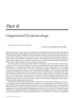
species abundance curves (Figure 22.1, upper panel) suggests the evenness with which individuals
are distributed among species (Tokeshi 1993). As will be shown shortly, evenness increases in the
following model sequence: geometric series < log series < discrete log normal < broken stick.
Although many models exist (Tokeshi 1993), abundance data are commonly fit to only four
models: logarithmic series, geometric series, discrete log normal, and broken stick. All have been
Species rank
Geometric series
Log normal
Broken stick
Log (number of individuals/species)
Least abundantMost abundant
Number of species/octave
Modal octave
Veil
line
Octave
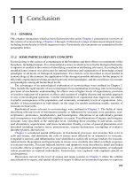
FIGURE 22.1 Species abundance curves for summarizing community data. The top panel depicts three
conventional models including the extremes (geometric series and broken stick) and most commonly used
(log normal) models. The bottom panel illustrates Preston’s (1948) approach to analyzing species abundance
data with a log normal model. Notice that there is a veil line on the x-axis. For most such curves, there
is some minimal count (e.g., one individual/species), below which abundance cannot be quantified. Much
of the mathematics associated with Preston’s analysis of the log normal model is associated with estimating
distributional parameters with such a left-truncated curve.
© 2008 by Taylor & Francis Group, LLC

Clements: “3357_c022” — 2007/11/9 — 18:31 — page 413 — #5
Biomonitoring and the Responses of Communities to Contaminants 413
interpreted in the context of resource competition, with the relative species abundance being used
to imply the portion of resources or niche volume secured by a species. Whether competition is
a reasonable foundation for such a model depends very much on the community, species assemblage,
or taxonomic group being studied. It may be very appropriate for studying an ecological guild but
quite inadequatefor acollectionof functionallydivergent species.Althoughtheexplanations basedon
realized niche and resource allocation “are useful in suggesting possibilities underlying community
organization” (Tokeshi 1993), interpretation based on competition theory should be done cautiously
(Hughes 1986). Some researchers prefer to view species abundance models as statistical models
because of this loose theoretical foundation. However, the cost of such freedom from theory is
a severely restricted ability to assign ecological meaning to results.
The simplest and earliest model, the geometric series (Motomura 1932), is based on the niche
preemption concept (Figure 22.1). According to this model, one species takes kth of the available
niche space, leaving only 1 −k for the remaining species to share. A second species then takes kth
of the remaining 1 −k niche space. This niche preemption sequence continues until all species have
secured their portion of the available niche space. Any variation from k among species is attributed
to stochasticity.
There will be a few very abundant species in such a community, as might be expected during
early stages of succession in which r-selected strategies dominate or for a community associated
with a severe environment in which one or a few factors determine species success (May 1976). The
associated model is given in the following equation (Magurran 1988):
N
i
= kN

1
1 −(1 −k)
s


[1 −k]
i−1
. (22.1)
A log series model is similar to the geometric series except that species arrive and occupy niche
space randomly, not in the regular intervals as described for the geometric series. The result is
a community with a few dominants and more rare species than the geometric model would predict.
The curve for the log series would be intermediate between the geometric series and log normal
models in Figure 22.1. The expected number of species with n individuals is αx
n
/n, with x being
a sample size-dependent constant less than 1 and α being a community-dependent constant. The
log series model is often described as the model most useful for “samples from small, stressed, or
pioneer communities” (Hughes 1986).
The discrete log normal model fits most communities (Magurran 1988) and is often advocated
as universally acceptable for species abundance modeling (May 1976). The competition theory
behind it is that a species’ success in occupying niche space is determined by many factors. The
result is more intermediate abundance species and fewer rare species than for the geometric series
model (Figure 22.1). In contrast to the geometric series model in which r-selection strategists often
dominate, this model might be more suggestive of equilibrium or K-selection strategies such as those
occurring in climax or unstressed communities.
The log normal model cannot be fit by simply calculating the central tendency and disper-
sion parameters, because values for some observations to the left of the veil point are not known
(Figure 22.1, lower panel). Preston (1948) speculated that log normal distributions were truncated
because of the difficulty sampling all rare species in a community and that the distribution would
shift to the right with larger sample sizes. Preston developed the classic method for analyzing the
truncated log normal species abundance curve by first separating all species into abundance classes.
The most convenient abundance categories were octaves, grouped by doubling in numbers such as
1 to 2, 2 to 4, 4 to 8, 8 to 16, 16 to 32, and so forth. The number of species in each octave was
plotted to produce a graph similar to the lower panel of Figure 22.1. The octaves are often labeled
relative to the modal octave (e.g., R = 0 denotes the modal octave, R =−1 denotes one octave to

© 2008 by Taylor & Francis Group, LLC
Clements: “3357_c022” — 2007/11/9 — 18:31 — page 414 — #6
414 Ecotoxicology: A Comprehensive Treatment
the left of the mode, and R = 2 denotes two octaves to the right of the mode). In samples containing
large numbers of species, a normal distribution is obtained when the log abundance of species is
plotted against the number of species in each category.
The original method of Preston (1948) or the more simplified approach of Newman (1995)
can be used to estimate the distribution parameters and subsidiary information such as the estim-
ated number of species in the community. The predicted number of species in octave R (S
R
)is
estimated from the number of species in the modal octave (S
0
) and the variance of the log normal
distribution, σ
2
.
Preston’s log normal distribution was found to be widely applicable for explaining the rank
abundance of many taxonomic groups. Although Preston did not provide an ecological explanation
for the generality of log normal distributions in nature, other ecologists discussed the evolutionary
implications. Using the broken stick model, MacArthur (1960) proposed that species abundance
distributions resulted from interspecific competition and allocation of resources among species.
According to this model, the niche space available to any species is allocated much as a length of
stick would be if a stick were randomly snapped along its length to produce S pieces. In more formal
terms, S −1 points are randomly identified along the length of the stick and the stick is broken at
these points. The length of each segment reflects the amount of niche space (inferred from species
abundance) allocated to each species. In such a model, the niche space would be randomly distributed
among the S species to produce a community with many moderately abundant species but relatively
few rare or extremely abundant species (Figure 22.1 bottom panel). As such, this model is most
likely to describe an equilibrium assemblage of very similar species (e.g., a specific guild in a climax

community).
Magurran (1988) provides estimators of the expected number of individuals (N
i
) for the ith most
abundant species (Equation 22.2) and the expected number of species (S
n
) for the nth abundance
class (Equation 22.3) based on the broken stick model:
S
n
= S
0
e
−(1/
√
2σ
2
)
2
R
2
, (22.2)
N
i
=
N
S
S

n=i

1
n
. (22.3)
Which specific model best fits the data statistically can be determined by deferring to the advice of
experts (e.g., May’s preference for the log normal model), or by applying conventional goodness-of-
fit methods. Magurran (1988), Ludwig and Reynolds (1988), and Newman (1995) provide the details
for formally assessing relative model goodness-of-fit. Regardless of how relative model goodness-
of-fit is examined, one is ultimately faced with the difficult task of deciding which model best fits
the ecological reality of the species assemblage being studied.
In general, attempts to seek underlying biological processes for log normal distributions were
unsuccessful. Recent analyses of log normal distributions and MacArthur’s broken stick model
have revealed their statistical inevitability (Gotelli and Graves 1996). Despite the lack of an evol-
utionary explanation, comparisons of the distribution of individuals among species are a powerful
tool in community ecology and ecotoxicology. Because of differences in sensitivity among spe-
cies, shifts in the relative abundance of tolerant and sensitive species at polluted sites should be
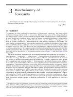
reflected in the shape of species abundance curves (Figure 22.2). As the classic example, Patrick
(1971) used the shapes of such curves to interpret shifts in diatom communities impacted by pol-
lution. Because the shape of the log normal distribution also reflects whether the contaminant is
toxic or has a stimulatory influence (e.g., nutrient enrichment), the curves could be employed
to distinguish between stressors. Thus, species abundance models extract more information than
simple species lists, but are applied much less frequently than diversity, evenness, and richness
metrics.
© 2008 by Taylor & Francis Group, LLC
Clements: “3357_c022” — 2007/11/9 — 18:31 — page 415 — #7
Biomonitoring and the Responses of Communities to Contaminants 415
Reference site
Contaminated site
0–1
1–2
2–4

4–8
8–16
16–32
32–64
64–128
128–256
256–512
512–1024
1024–2048
0
10
20
30
40
50
60
Number of individuals per species
Number of species
FIGURE 22.2 The predictedrank abundancedistributionof speciescollected from referenceand pollutedcom-
munities (Preston 1948). The figure shows the number of species within each abundance class. The community
from the reference site approximates a log normal distribution, whereas the community from the contaminated
site is characterized by lower richness and increased abundance of tolerant species. This is a typical response
of algal and benthic macroinvertebrate communities to organic pollution.
22.3.2 THE USE OF SPECIES RICHNESS AND DIVERSITY TO
CHARACTERIZE COMMUNITIES
22.3.2.1 Species Richness
As noted in Chapter 21, patterns of species richness across local, regional, and global scales have
intrigued community ecologists for several decades. Community ecotoxicologists have routinely
employed species richness as an indicator of ecological integrity. Rapport et al. (1985) include
reduced species richness as one of five general indicators of the “ecosystem distress syndrome”

(Chapter 25). Among the scores of measures used by community ecotoxicologists to assess effects
of contaminants, reduced species richness is probably the most consistent (and least controversial)
response. Because of the perceived value of biodiversity to the lay public, measures of species
richness also have high societal relevance.
Species richness is defined as the number of species present in a prescribed sampling unit.
Richness (R) can be determined by sampling more and more individuals from a site and keeping
a running tally of the number of species that appear (Equations 22.4 and 22.5). The results can be
used to estimate the total number of species in the community. Plots of the cumulative number of
species versus sampling effort (e.g., number of dredge hauls, km
2
searched, biomass sampled, or
number of individuals captured) will show an initial rapid increase in the number of species followed
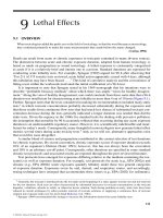
by a more gradual increase until becoming asymptotic (Figure 22.3). In most situations, this measure
of species richness can be quite difficult to determine. In others, it might be undesirable to do such
exhaustive sampling of a community if sampling was destructive or disruptive.
The number of species in a community can also be approximated with specific models (e.g., a log
normal model) or indices that assume specific models linking sample size (number of individuals
in the sample or N) and species richness (Equations 22.4 and 22.5) (Ludwig and Reynolds 1988,
Magurran 1988, Matthews et al. 1998). All of these methods rely on the law of frequencies (Fisher
et al. 1943), which holds that a relationship exists between the number of species and number
of individuals in any ecological community. However, the law of frequencies does not dictate
© 2008 by Taylor & Francis Group, LLC
Clements: “3357_c022” — 2007/11/9 — 18:31 — page 416 — #8
416 Ecotoxicology: A Comprehensive Treatment
Sampling effort
Asymptotic estimate of species richness
150
100
50
0

Cumulative number of species
FIGURE 22.3 Estimation of species richness for a community with a cumulative number of species versus
sampling effort curve.
a particular relationship between the numbers of species and individuals. Thus, LudwigandReynolds
(1988) argue that, unless shown to be true, the assumption of a specific relationship between S and
N in these models or metrics should be handled cautiously:
R
Margalef
=
S − 1
ln N
, (22.4)
R
Menhinick
=
S
√
N
. (22.5)
Despite broad support for the use of species richness to assess biological integrity, estimating the
number of species in the field is often problematic. Except in a few examples where all species in
a habitat can be completely sampled (e.g., bird communities on small islands), we rarely know the
total number of species in a community. Furthermore, species richness is highly dependent on area
(Chapter 21) and increases asymptotically with sample size and the number of individuals collected
(May 1973). Consequently, comparisons of the number of species amongsitesshouldbe standardized
for area and number of individuals (Vinson and Hawkins 1996). This is not a serious limitation
in most biomonitoring studies because the same sampling effort will presumably be employed in
both reference and impacted sites; however, it does complicate making comparisons with historic
data or comparing results from different studies. One proposed solution to this problem is the use
of a procedure known as rarefaction (Simberloff 1972), in which samples are selected randomly

from the entire dataset to derive a quantitative relationship between number of species and total
abundance. Rarefaction procedures estimate the expected number of species based on samples with
standard sample sizes. The advantage of the rarefaction estimate is that samples of different sizes
can be compared. The disadvantage is that information is lost when the actual sample size taken at
a site is larger than the sample size for which the number of species is being estimated. The equation
for estimating species richness by rarefaction is:
ˆ
S
n
=
S

i=1
1 −

N −N
i
n


N
n

, (22.6)
where N = the number of individuals in the sample, N
i
= the number of individuals of species
i in the sample, S = the number of species in the sample, and n = the sample size (number of
individuals) to which normalization is being done.
© 2008 by Taylor & Francis Group, LLC

Clements: “3357_c022” — 2007/11/9 — 18:31 — page 417 — #9
Biomonitoring and the Responses of Communities to Contaminants 417
A second more pervasive problem is that measures of species richness do not account for dif-
ferences in abundance among species. Theoretically, two locations could have very different total
abundances and a very different distribution of individuals among species and still have the same
species richness. Measures of species diversity, which account for both richness and the distribution
of individuals among species, have been developed to resolve this problem. Although used routinely
to compare communities in different locations, most diversity measures have received intense criti-
cism from ecologists and ecotoxicologists. Diversity indices have been attacked based on theoretical,
statistical, and conceptual arguments (Fausch et al. 1990, Green 1979, Hurlbert 1971). Despite the
criticism, diversity measures continue to be widely used in biomonitoring studies and have appeared
to multiply in the literature.
22.3.2.2 Species Diversity
Many ecologists, including ecotoxicologists, condense large species abundance data sets into
diversity indices. There are two general types of diversity indices, those based on dominance and
those derived from information theory. Both types include a species richness component and an
evenness component of diversity; however, the relative importance of rare species differs between
the two approaches. Simpson’s index (1949), the most widely used measure of dominance, is
given as
ˆ
λ =
S

i=1
1
p
2
i
, (22.7)
where λ is the measure of diversity and p

i
is the proportion of the ith species in the sample.
The value of λ ranges from 1 to S (where S = species richness), with larger values represent-
ing greater diversity. Community evenness reflects the distribution of individuals among species.
If all species in a community have the same relative abundance, the value of λ is maximized
and equals species richness. In practice, Equation 22.8 is often used to avoid bias associated
with estimating p
i
with N
i
/N and from diversity estimation for the entire community based on
a sample:
λ =
S

i=1
N
i
(N
i
−1)
N(N −1)
. (22.8)
Simpson’s modified index as given in Equation 22.8 is converted in practice to 1 − λ so that
any increase in the index reflects an increase in diversity. This weighted mean of the species
proportions is very sensitive to dominant species and relatively insensitive to rare species. Thus,
the main criticism of Simpson’s index is that rare species contribute relatively little to the index
value.
Two common diversity indices based on information theory, the Shannon–Wiener and Brillouin
indices, are more sensitive to rare species (Qinghong 1995) and, in our opinion, are more relevant

to ecotoxicology. The distinction between the two indices is simply that the Shannon–Wiener index
(Equation 22.9) estimates diversity for the community from which the sample was taken, whereas
Brillouin’s index (Equation 22.10) estimates diversity for the sample itself. The Shannon–Wiener
index can be described as the uncertainty of predicting the species of a randomly selected individual
from the community. This uncertainty increases as more species are present in the community and
as the individuals are more evenly distributed among those species (Ludwig and Reynolds 1988).
Although calculated here using natural logarithms, both diversity indices can be calculated with
© 2008 by Taylor & Francis Group, LLC
Clements: “3357_c022” — 2007/11/9 — 18:31 — page 418 — #10
418 Ecotoxicology: A Comprehensive Treatment
base 10 or 2. Therefore, it is important to note units in published diversity (and related evenness)
indices before using them together.
H

=−
S

i=1
p
i
ln p
i
∼
=
−
S

i=1
N
i

N
ln

N
i
N

(22.9)
H =
1
N
ln
N!

S
i=1
N
i
!
(22.10)
In Equations 22.9 and 22.10, the units of diversity are units of information per individual.
If log
10
or log
2
were applied, the units would have been decits/individual or bits/individual, respect-
ively. Like Simpson’s index, Shannon–Wiener diversity is maximized (H
MAX
) when all species are
equally abundant in a sample.

22.3.2.3 Species Evenness
How equally the individuals in a community are distributed among the species can be measured with
a variety of indices. The first two to be illustrated (Pielou 1969) are based on H

and H. They are
simply H

or H divided by their estimated maxima, and consequently, the resulting evenness indices
are those for the entire community (J

) or for the sample itself (J). The maxima are used because
they would be the values for H

and H if individuals were uniformly distributed among the available
species:
J

=
H

ln S
(22.11)
J =
H
H
MAX
. (22.12)
H
MAX
is defined by the following formula:

H
MAX
=
1
N
ln

N!
([N/S]!)
S−r
{[(N/S) +1]!}
r

,
where [N/S]=the integer part of the quotient, N/S, and r = N −S[N/S] (Magurran 1988).
The third evenness index (Alatalo 1981) is insensitive to species richness and combines
both Hill’s and Shannon–Wiener’s indices (Equation 22.13). It is a modification of Hill’s index
([1/λ]/[e
H

]), a measure that quantifies the proportion of common species in the sample. In the
modified Hill’s index, e
H

reflects the number of abundant species and 1/λ reflects the number of
very abundant species. The modification consists only of subtracting the maxima (i.e., 1) from each
of the estimates, 1/λ and e
H

:

E =
(1/
ˆ
λ) −1
e
H

−1
. (22.13)
22.3.2.4 Limitations of Species Richness and
Diversity Measures
The Simpson, Shannon–Wiener, and Brillouin indices are three examples from a long list of diversity
measures that have been employed by community ecotoxicologists to assess effects of contaminants.
Studies comparing performance and sensitivity of diversity measures have shown that each has
© 2008 by Taylor & Francis Group, LLC
Clements: “3357_c022” — 2007/11/9 — 18:31 — page 419 — #11
Biomonitoring and the Responses of Communities to Contaminants 419
4 Species, even
distribution
5 Species, even
distribution
5 Species, uneven
distribution
10 Species, uneven
distribution
Community A Community B Community C Community D
0
1
2
3

4
5
6
Diversity, evenness
Simpson’s
diversity
Shannon–Wiener
diversity
Evenness
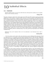
FIGURE 22.4 The influence of species richness and evenness on Shannon–Wiener and Simpson’s diversity
in four communities. The pie diagrams show the relative abundance of each species in the community. Note
that both measures of diversity increase as species richness and evenness increase.
specific limitations (Boyle et al. 1990). Thus, it is not possible to recommend an index that will be
useful in all situations. Indices that are sensitive to dominant species will be more appropriate when
stressors, such as organic enrichment, favor a particular group. In contrast, because rare species are
often the first to be eliminated from polluted sites, it may be more appropriate to employ an index
sensitive to rare species when assessing effects of toxic chemicals.
The dependence of the Shannon–Wiener diversity index on both species richness and evenness
is considered a serious shortcoming by some researchers (Qinghong 1995). Because decreases in
species richness can be offset by increases in evenness (or vice versa), a single value of H

can be
derived from numerous combinations of richness and evenness values. For example, in Figure 22.4,
diversity (H

) is the same (1.61) in two hypothetical communities (B and D), despite large differences
in species richness and evenness. In practical terms, this means that changes in species diversity may
go undetected even though large shifts in community composition have occurred. To address this
problem, Qinghong (1995) proposed a simple model of species diversity that expresses changes in
richness and evenness graphically (Figure 22.5). Using this approach, differences between any two

points (e.g., two sampling locations or two points in time) on a plot of diversity versus richness
can be attributed to a change in diversity, richness, or evenness.
The most serious criticism of simple community-level endpoints such as species richness and
diversity is the loss of information that occurs when details of community composition are aggreg-
ated in a single number. While species abundance plots such as those developed by Preston (1948)
describe how individuals are distributed among species (Figure 22.1), they do not provide inform-
ation on community composition. Because sensitive species may be replaced by tolerant species at
contaminated sites, it is conceivable that two communities could have a strikingly different com-
position but still have similar richness and diversity. An alternative approach that retains important
information about communitycompositionrelevant to contaminants is theuseof biotic indices. These
indices (Section 22.3.3) are designed to integrate estimates of relative abundance with measures of
species-specific sensitivity, thus capturing in a single index the fraction of a community consisting
of tolerant and sensitive organisms.
© 2008 by Taylor & Francis Group, LLC
Clements: “3357_c022” — 2007/11/9 — 18:31 — page 420 — #12
420 Ecotoxicology: A Comprehensive Treatment
Evenness
Maximum evenness and diversity
Log(2) species richness
Species diversity (H′ )
A
B
FIGURE 22.5 Illustration showing the diversity monitoring (DIMO) model (Qinghong 1995), an alternative
approach for presenting species richness, evenness, and Shannon–Wiener diversity in communities. The diag-
onal line is the maximum species diversity and evenness based on species richness within a community. The
two points represent the species diversity and richness of two different communities (A and B). The angle of
the vector for each point represents the evenness component of the Shannon–Wiener diversity index. In this
hypothetical example, community B has greater species richness but lower species diversity than community
A because of the lower evenness.
Community ecologists have recently begun to appreciate the importance of rare species

(e.g., those species that occur at low densities or are infrequently encountered in a community),
especially in terms of preservation of biological diversity. However, the importance of rare species
in ecotoxicology and bioassessment has received little attention (Cao et al. 1998, Fore et al. 1996).
Barbour and Gerritsen (1996) argue that it is unnecessary and would be fiscally prohibitive to include
rare species in biological monitoring programs. For practical reasons and because of the assumption
that rare species contribute relatively little to ecosystem function, a common practice in biological
assessments is to remove rare species from data analyses. However, becauserarespecies may account
for a disproportionate number of the total species at undisturbed sites (Gotelli and Graves 1996),
removing them from the analysis may decrease our ability to detect differences among locations.
In addition, rare species are more prone to local extinction because of low population densities.
Finally, recent studies conducted in aquatic systems indicate that censoring data to eliminate rare
species may underestimate effects of anthropogenic perturbations. Cao et al. (1998) showed that
differences between reference and impacted sites were reduced if rare species were removed from
the analyses (Figure 22.6). These researchers also showed that the small sample sizes typical of
most biomonitoring studies often miss rare species, resulting in greater underestimation of species
richness at reference sites compared to polluted sites.
22.3.3 BIOTIC INDICES
Measures of total abundance, diversity, and species richness may not respond to some types of
anthropogenic perturbations if sensitive species are simply replaced by tolerant species. Because
sensitivity to contaminants often varies among species, the relative abundance of sensitive and
tolerant taxa in a community could be employed to assess the degree of contamination. Biotic
indices were developed early in the history of ecotoxicology with the intent of assessing the state
of a community based on abundance of sensitive and tolerant species. Although Matthews et al.
(1998) note the subjective nature of many tolerance rankings and the existence of different rankings
© 2008 by Taylor & Francis Group, LLC
Clements: “3357_c022” — 2007/11/9 — 18:31 — page 421 — #13
Biomonitoring and the Responses of Communities to Contaminants 421
Sample size
Species richness
(a) All species included

(b) Rare species deleted
Species richness
Reference
Moderately impacted
Severely impacted
Reference
Moderately impacted
Severely impacted
FIGURE 22.6 The relationship between sample size and species richness at reference, moderately impacted
and severely impacted sites when all species are included (a) and when rare species are deleted (b). Because
rare species often comprise a greater portion of communities at reference sites, the difference between ref-
erence and impacted sites diminishes when rare species are deleted. (Modified from Figure 2 in Cao et al.
(1998).)
for the same species used in different regions, they conclude that biotic indices are used effectively
throughout Europe today.
Innumerable biotic indices exist (Matthews et al. 1998), and all have similar features. Biotic
indices assign values to individual taxa based on their relative sensitivity or tolerance to a specific
type of pollution. These values are often generated based on expert opinion of ecologists with
knowledge of the communities being impacted. This approach allows more information and the
most relevant information to be combined in comparison to the simple diversity, evenness, and
richness indices discussed earlier. However, it also makes subjective the selection of particular
community qualities and the assignment of scores or weights to these qualities. In addition, the
indices are relative. A score from a site suspected of being impacted is meaningful only relative
to the score expected for an unimpacted site. Finally, and as a consequence of the previous points,
the indices tend to be useful in a limited context, and must be modified thoughtfully to be applied
elsewhere.
Because biotic indices account for both species-specific sensitivity and relative abundance, they
are strongly influenced by pollution-induced changes in community composition. For example, it is
well established that mayflies (Ephemeroptera), caddis flies (Trichoptera), and stoneflies (Plecoptera)
are relatively sensitive to organic enrichment, whereas chironomids (Diptera) are generally tolerant.

Indices such as Hilsenhoff’s Biotic Index (Hilsenhoff 1987) take advantage of these differences in
sensitivity and categorize sites based on the relative abundance of sensitive and tolerant species.
© 2008 by Taylor & Francis Group, LLC
Clements: “3357_c022” — 2007/11/9 — 18:31 — page 422 — #14
422 Ecotoxicology: A Comprehensive Treatment
Hilsenhoff’s biotic index is given as
Biotic Index = p
i
/t
i
(22.14)
where p
i
and t
i
are the proportion abundance and tolerance values of the ith species, respectively.
Because most biotic indices use estimates of relative abundance, quantitative sampling is not neces-
sary to calculate these measures. This feature is particularly useful for rapid bioassessment protocols
(RBPs) (see Section 22.4) that often rely upon qualitative measures of community composition.
Because biotic indices are based on differences in species-specific sensitivity, their usefulness
is often restricted to the particular region where tolerance values (t
i
) were developed. Hilsenhoff’s
biotic indexuses species-specifictolerancevalues frommore than2000macroinvertebrate collections
from polluted and unpollutedWisconsin streams. Depending on the amount of variation in sensitivity
among species within a family or higher taxonomic unit, pollution indices based on coarse levels of
taxonomic resolution may be an effective solution to regional specificity. Chessman (1995) showed
that family-level tolerance values were necessary for Australian streams because of the lack of
taxonomic keys and the difficulty identifying immature life stages for some groups. A modified
version of Hilsenhoff’s biotic index based on family-level estimates of tolerance provided reasonable

estimates of biological condition and was appropriate as an initial screening approach for water
quality assessments (Hilsenhoff 1988).
Another criticism of pollution indices is that they are often specific to a particular class of con-
taminants (Chessman and McEvoy 1998, Slooff 1983). While Hilsenhoff’s biotic index is especially
well suited for assessing impacts of organic enrichment, the applicability of this index to other
classes of contaminants (e.g., heavy metals, acidification, or pesticides) is uncertain. From a prac-
tical perspective, chemical-specific pollution indices may be of little value in systems affected by
multiple chemical stressors. An alternative approach is to develop biotic indices that respond to
more general classes of perturbations. Lenat (1993) published an extensive list of tolerance values
for benthic macroinvertebrates in North Carolina (USA) streams. Unlike other pollution indices,
Lenat’s North Carolina Biotic Index (NCBI) is intended to provide a more general assessment of
water quality, regardless of pollution type. Comparisons of species-specific tolerance values from
Hilsenhoff’s biotic index and the NCBI revealed many differences; however, mean tolerance values
for major taxonomic groups were similar (Lenat 1993). These results are encouraging and suggest
that sensitivity of some groups may be independent of the type of perturbation.
Akeyadvantageof developingchemical-specificbiotic indicesisthe potential toidentify stressors
based on biological measures. Chessman and McEvoy (1998) proposed a suite of biotic indices,
each responding to a particular type of perturbation. A diagnostic index, based on family-level
responses, was developed for several types of physical and chemical perturbations. Chessman and
McEvoy (1998) concluded that, while diagnostic indices had promise, differences in sensitivity
among species within a family hindered their performance. If chemical-specific biotic indices can be
developed, these indices may be useful for quantifying the importance of individual chemicals in
systems receiving multiple stressors (Box 22.1).
Box 22.1 Experimental Determination of Species-Specific Sensitivity
Perhaps the most serious criticism of biotic indices concerns the subjective assignment of tol-
erance values to individual species (Clements et al. 1988, 1992, Herricks and Cairns 1982,
Matthews et al. 1998). While best professional judgment applied to survey data can provide
legitimate estimates of species-specific sensitivity, these data should be supported by experi-
mental evidence. In a review of biomonitoring approaches, Johnson et al. (1993) recognized
the need to integrate laboratory-derived tolerance values with field data. The subjectivity and

tautological reasoning inherent in biotic indices could be avoided by validating tolerance values
© 2008 by Taylor & Francis Group, LLC
Clements: “3357_c022” — 2007/11/9 — 18:31 — page 423 — #15
Biomonitoring and the Responses of Communities to Contaminants 423
Species 1, slope = 0.08
Species 2, slope = 0.40
010203040506070
0
20
40
60
80
100
Chemical concentration
Percent mortality
Species 3, slope = 0.91
Species 4, slope = 1.4
FIGURE 22.7 Results of community-
level toxicity tests comparing the hypo-
thetical responses of four species to
a contaminant. Theslope of the relationship
between percent mortality and concentra-
tion is an indicator of relative sensitivity to
the chemical andcan beusedin thedevelop-
ment of biotic indices. In this example, spe-
cies 1 is relatively tolerant to the chemical
whereas species 4 is highly sensitive.
experimentally. Because of the opportunity to test responses of numerous species to the same
chemical or mixture of chemicals simultaneously, community-level toxicity tests conducted in
microcosms or mesocosms are an efficient way to obtain species-specific estimates of sensit-

ivity. Standard toxicological endpoints (e.g., LC50, EC50) could be used to estimate relative
sensitivity among species in a mesocosm experiment. Alternatively, experimental designs that
use regression analyses to establish concentration–response relationships can provide objective
estimates of species-specific sensitivity for numerous taxa (Figure 22.7). Estimates of relative
sensitivity to chemicals derived experimentally could be integrated with field measures of relat-
ive abundance to produce pollution indices for different classes of contaminants. Clements et al.
(1992) used this approach to develop an index of community sensitivity for benthic macroin-
vertebrates in metal-polluted streams. Benthic macroinvertebrate communities collected from
a reference site were exposed to heavy metals in stream microcosms. Experimentally derived
estimates of relative sensitivity were integrated into a biotic index (the index of metals impact),
which was used to evaluate the degree of metal pollution downstream from the input of metals
in a natural system.
In summary, while biotic indices have been employed extensively in European and other
countries, they have received considerably less attention in the United States. These indices
have been most successful when limited to a single class of stressors, especially organic enrich-
ment. It should not be surprising when indices based on sensitivity to one chemical stressor
fail to distinguish other types of perturbation. Bruns et al. (1992) rated several biological
indicators based on their ecosystem conceptual basis, variability, uncertainty, ease of use, and
cost-effectiveness. Litter decomposition and taxonomic richness received the highest ratings,
whereas a biotic index received the lowest rating, primarily because it lacked information on
responses of taxa to specific chemical toxicants. Finally, it is important to remember that the
presence of tolerant taxa or the absence of sensitive taxa may result from numerous factors
other than contaminants (Cairns and Pratt 1993). Biotic indices in isolation cannot demonstrate
effects of pollution, only that a site is dominated by pollution-tolerant or pollution-sensitive
organisms. However, biotic indices could be employed to evaluate potential reference sites in
biomonitoring studies. A community dominated by species that are sensitive to a particular
chemical provides reasonable evidence for the absence of that chemical.
22.4 DEVELOPMENT AND APPLICATION OF RAPID
BIOASSESSMENT PROTOCOLS
One frequent criticism of community-level biomonitoring studies is the high cost of these approaches

compared to physicochemical measures or single species toxicity tests. Because of the patchy spatial
© 2008 by Taylor & Francis Group, LLC
Clements: “3357_c022” — 2007/11/9 — 18:31 — page 424 — #16
424 Ecotoxicology: A Comprehensive Treatment
distribution of natural populations and the resulting high variability, large numbers of replicate
samples are often necessary to detect differences between reference and contaminated sites. The
time required for sample processing and species-level identification of taxonomically difficult groups
may also beprohibitive, particularly foragencies conducting large-scalemonitoringprograms. Niemi
et al. (1993) compared the cost and explanatory value of physical, chemical, and biological meas-
ures of recovery rates in streams. Biological measures (e.g., density, primary production, leaf litter
decomposition) were considerably more expensive because of the greater variability and the need
to collect large numbers of replicate samples. However, these authors acknowledged that because
of their greater explanatory power, high cost should not preclude the use of biological variables in
ecological assessments. We should also note that some studies have reported that costs of biolo-
gical monitoring were competitive with other approaches for assessing water quality. An analysis
conducted by the Ohio Environmental Protection Agency (EPA) showed that per sample costs of
invertebrate and fish surveys were actually less than physical and chemical analyses of water quality
(Karr 1993).
While there is evidence that biological assessments can be conducted cost-effectively, it is likely
that the expense and logistical difficulties of conducting these surveys has limited our ability to
assess the status of communities at larger spatial scales. Resolving the often conflicting goals of
large-scale, spatially extensive monitoring with the need for intensive, long-term biological assess-
ments requires innovative techniques that will improve efficiency but not sacrifice data quality. Rapid
assessment programs (RAPs) and their aquatic counterparts, RBPs, were developed independently
in the fields of conservation biology and biomonitoring to address these concerns. Both approaches
attempt to streamline biological assessments by employing a variety of cost-saving but somewhat
controversial procedures. Rapid assessment programs have been used extensively in conservation
biology, especially in tropical ecosystems, where researchers must quickly estimate biodiversity and
prioritize sites for preservation without the luxury of exhaustive biological surveys. The validity
of many of these programs is based on the assumption that diversity of one group of organisms

can be used as an indicator of total biological diversity within a region. For example, conser-
vation biologists have used surveys of well-known flora and fauna (flowering plants, birds, and
mammals) to estimate diversity of more difficult taxonomic groups (invertebrates). Using species
diversity of one group to predict diversity of other groups has intuitive appeal and could signi-
ficantly reduce costs of biological surveys (Blair 1999); however, the underlying assumption that
diversity across broad taxonomic groups is regulated by the same ecological processes remains to be
tested.
Innovations in rapid bioassessment procedures that streamline biological monitoring programs
and reduce costs have accelerated the development of several large-scale monitoring programs in the
United States, including the U.S.EPA’sEnvironmentalMonitoring andAssessmentProgram (EMAP)
and the U.S. Geological Survey’s National Water-Quality Assessment (NAWQA) program (Resh
et al. 1995). The long-term goals of these programs are to assess the status and trends of terrestrial and
aquatic ecosystems using a combination of probabilistic sampling designs and large-scale (regional)
analyses. Given the limited funds available for routine monitoring in the United States, it is unlikely
that these programs could accomplish their objectives without the cost savings provided by RBPs.
More importantly, the reduced collection and processing costs allow researchers to sample a larger
number of sites or increase the frequency of sampling.
In aquatic ecosystems, RBPs reduce sample collection and processing costs by (1) using qualit-
ative sampling techniques, (2) subsampling and fixed-count processing, (3) eliminating replication
and pooling samples collected from individual sites, and (4) relaxing the level of taxonomic resolu-
tion (Plafkin et al. 1989, Resh and Jackson 1993). Each of these four cost-saving measures involves
important trade-offs that must be considered when implementing biomonitoring programs, regard-
less of whether sampling is conducted within a single stream or at a regional level. Resh et al. (1995)
acknowledged the widespread acceptance of these cost-saving measures, noting that in our haste to
expand biomonitoring programs, the consequences of reduced data quality have not been critically
© 2008 by Taylor & Francis Group, LLC
Clements: “3357_c022” — 2007/11/9 — 18:31 — page 425 — #17
Biomonitoring and the Responses of Communities to Contaminants 425
evaluated. In a review of RPBs, Hannaford and Resh (1995) reported that, while RBPs may be
appropriate for prioritizing sites, their ability to produce legally defensible data or for routine impact

assessments remains questionable. Later, we consider the limitations of each of the cost-saving
measures used in RBPs.
22.4.1 APPLICATION OF QUALITATIVE SAMPLING TECHNIQUES
The abandonment of quantitative sampling techniques in many RBPs is an issue that requires ser-
ious consideration. Because of the time required to process quantitative samples, especially those
collected from aquatic habitats, qualitative surveys of community composition have become increas-
ingly common in biological assessments. Qualitative sampling techniques generally limit our ability
to express data in terms of numbers of organisms per unit area or volume. Because interactions
that structure communities are determined largely by absolute numbers of organisms and not their
relative abundance, qualitative assessments do not provide insight into factors that regulate com-
munity composition. Furthermore, statistical analyses of biomonitoring results based on qualitative
or quantitative data may lead to important differences. Figure22.8showsresponsesofseveralbenthic
macroinvertebrate metrics to heavy metals and compares statistical results based on qualitative (relat-
ive abundance) or quantitative (number/m
2
) data. Analyses based on qualitative data were generally
more variable and often unable to detect differences between metal-polluted and unpolluted sites.
To be fair, our appraisal of qualitative sampling employed in many RBPs neglects one major
advantage of this approach. Because sample-processing times are greatly reduced using qualitative
techniques, organisms can be collected from a larger and more diverse group of microhabitats.
Sampling diverse habitats generally increases the total number of species collected compared to
traditional quantitative techniques (e.g., 0.1 m
2
Surber sampler), which are often microhabitat-
specific. Thus, specieslistsgenerated from qualitative sampling of diverse habitats will likelyprovide
a more complete characterization of total species richness. Although quantitative techniques can be
modified to sample different microhabitats, care must be taken to estimate relative habitat availability
and to express the data accordingly.
22.4.2 S
UBSAMPLING AND FIXED-COUNT SAMPLE PROCESSING

The second major cost-saving measure in RBPs is the use of fixed-count sample processing
(e.g., removal of 100, 200, or 300 individuals from a sample). Although fixed-count processing
is standard in most RBPs, few studies have critically examined this procedure or determined the
optimal number of individuals that should be removed from a sample (Barbour and Gerritsen 1996,
Courtemanch 1996, Somersetal. 1998, Vinson and Hawkins1996). Courtemanch (1996) argues that,
because of the relationship between total abundance and species richness, fixed-count processing of
samples can result in inconsistent and erroneous estimates of species richness. In addition, fixed-
count processing is biased against rare taxa (although fixed counts can be supplemented by including
large, rare taxa). Barbour and Gerritsen (1996) defend the use of fixed-count subsampling on the
basis of significantly reduced costs and, more importantly, a greater ability to detect differences
among sites compared to analyses using entire samples. Surprisingly, some studies have reported
that removing a larger number ofanimalsfrom samples does not necessarily improvetheperformance
of RBP metrics. Using data collected from lakes, Somers et al. (1998) concluded that a two or three
times increase in the number of organisms subsampled by fixed-count processing did not improve
the ability of metrics to distinguish among locations. Analysis of more than 2000 benthic macroin-
vertebrate samples collected from the United States showed that, while fixed-count processing will
significantly underestimate true species richness, this technique is quite robust with respect to dis-
tinguishing among locations (Vinson and Hawkins 1996). Furthermore, these authors conclude that
fixed-count subsampling eliminates the need for using rarefaction techniques to estimate species
richness when density varies greatly among locations.
© 2008 by Taylor & Francis Group, LLC
Clements: “3357_c022” — 2007/11/9 — 18:31 — page 426 — #18
426 Ecotoxicology: A Comprehensive Treatment
Quantitative Qualitative
EPT
Total ephemeroptera
Total plecoptera
Heptageniidae
Rhyacophilidae
Predators

Scrapers
0
1
2
3
4
5
6
F-value
***
***
***
***
***
**
**
*
*
EPT
Total ephemeroptera
Total plecoptera
Heptageniidae
Rhyacophilidae
Predators
Scrapers
Variable
Variable
r
2
0

.1
.2
.3
.4
.5
FIGURE 22.8 Comparison of quantitative (number/m
2
) and qualitative (relative abundance) measures of
macroinvertebrate community responses to metals in Rocky Mountain streams. Data were obtained from one-
way ANOVA testing for differences among reference, moderately polluted, and highly polluted streams. All
measures based on quantitative data were highly significant (
∗
P < .05;
∗∗
P < .001;
∗∗∗
P < .0001), whereas
only two measures based on qualitative data (EPT and scrapers) were significant. In all instances, F-values and
the amount of variation explained were much greater when based on quantitative measures. (From Clements,
unpublished results.)
22.4.3 POOLING SAMPLES
The third cost-saving measure common to many RBPs is the collection of a single, unreplicated
sample from reference and polluted sites. The abandonment of replication has been criticized because
it precludes estimating within-site variationandthereforelimits statistical analyses (Resh et al. 1995).
Although one could argue that since RBPs often integrate numerous metrics, each reflecting a unique
component of ecological integrity, rigorous statistical analyses are less important. Indeed, summary
metrics in RBPs are generally compared among sites without including estimates of variation. How-
ever, just like their constituent metrics, RBPs can vary among locations due to chance alone and
therefore some analysis of variation would be useful.
From an experimental design perspective, the uneasiness that some ecotoxicologists feel about

the abandonment of replication in RBPs may be irrelevant. Because samples collected from a single
site are not true replicates, some argue that the use of inferential statistical analyses is not appropriate
© 2008 by Taylor & Francis Group, LLC
Clements: “3357_c022” — 2007/11/9 — 18:31 — page 427 — #19
Biomonitoring and the Responses of Communities to Contaminants 427
(Hurlbert 1984). One practical solution to the lack of replication in RBPs is to collect data from many
reference and polluted sites within a region (Clements and Kiffney 1995, Feldman and Connor 1992).
Using this approach, sites are placed into categories (e.g., reference or impacted) and estimates
of variation within and between categories are compared. This approach is the basis for the use
of regional reference conditions described in Section 22.5. Because of the patchy distribution of
organisms at any one location, it is recommended that collecting several pooled samples from a site
is better than one large sample of equal area (Vinson and Hawkins 1996).
22.4.4 RELAXED TAXONOMIC RESOLUTION
The appropriate level of taxonomic resolution is an important consideration in any biomonitoring
study because of the difficulty and cost associated with identifying organisms to species. For many
groups oforganismsandin some regions, species-level identificationis impossible becauseofthe lack
of sufficient taxonomic keys (e.g., many invertebrate groups in the tropics), difficulties with imma-
ture life stages (e.g., most aquatic insects), and large numbers of undescribed species (e.g., fungi,
nematodes, and tropical beetles). Because of the difficulty in obtaining species-level identifications,
some researchers have proposed abandoning traditional taxonomic approaches in favor of “recog-
nizable taxonomic units” (RTUs) for assessing biological diversity. RTUs are taxa that are readily
distinguished based on simple morphological characteristics and are generally developed by indi-
viduals who lack formal training in taxonomy. Oliver and Beattie (1993) reported that estimates of
biodiversity of spiders, ants, and mosses based on RTUs were similar to those based on traditional
taxonomic analysis (Figure 22.9). The correspondence for marine polychaetes was not as good, sug-
gesting that applicability of RTUs for biomonitoring must be evaluated on a group-by-group basis.
Although these nontaxonomic approaches can significantly reduce sample-processing costs, the lack
of taxonomic information may hinder comparisons among studies.
Taxonomic resolution is a serious issue that deserves special consideration when employing
RBPs. Large savings in sample-processing costs may be realized using relatively coarse (e.g., family

level) taxonomic resolution (Lenat and Barbour 1994, Vanderklift et al. 1996). The major assump-
tion when employing relaxed taxonomic resolution is similar to that of studies using species-level
Spiders Ants Polychaetes Mosses
0
20
40
60
80
100
Group
Number of species or RTUs
Species
richness
RTUs
FIGURE 22.9 Comparison of species richness and RTUs forspiders, ants, polychaetes, and mosses. Measures
of species richness were determined by taxonomic experts, whereas RTUs were determined by technicians with
minimal training in taxonomy. Results show that for most groups, actual species richness and RTUs were
similar. The major exception was for marine polychaetes, which were split into more groups by nonexperts.
(Data from Table 1 in Oliver and Beattie (1993).)
© 2008 by Taylor & Francis Group, LLC
Clements: “3357_c022” — 2007/11/9 — 18:31 — page 428 — #20
428 Ecotoxicology: A Comprehensive Treatment
identification, namely, that these taxonomic units respond predictably to environmental gradients
(Olsgard et al. 1998). Several researchers have reported that relatively coarse levels of taxonomic
resolution are sufficient to detect effects of pollution (Ferraro and Cole 1995, Olsgard et al. 1998,
Vanderklift et al. 1996, Warwick 1993). For example, Bowman and Bailey (1997) concluded that
patterns of community structure were similar when analyses were based on genus- or family-level
identifications. Aggregate measures of phytoplankton community composition were actually more
reliable indicators of eutrophication than species-level analyses in a whole-lake enrichment exper-
iment (Cottingham and Carpenter 1998). Marchant et al. (1995) reported that analyses of benthic

macroinvertebrate data collected over a large region were relatively robust to sampling techniques
and taxonomic resolution. They showed that patterns of benthic communities measured using qual-
itative sampling techniques (presence/absence data) and family-level identification were similar to
those using quantitative data and species-level identification. Ferarro and Cole (1995) compared the
ability of different indices to detect differences between polluted and unpolluted locations when ana-
lyses were conducted at the level of genus, family, order, and phylum. Results showed that the level
of taxonomic resolution was relatively unimportant for detecting pollution. The most likely explana-
tion for these results is that taxonomically related species often have similar ecological requirements
and similar sensitivities to contaminants (Warwick 1988).
As previously noted, conservation biologists have also investigated the consequences of relaxed
taxonomic resolution on their ability to estimate biological diversity. Williams and Gaston (1994)
found that family-level richness was a highly significant predictor of species richness (r
2
> .79) for
several groups, including ferns, butterflies, passerine birds, and bats. However, these researchers
cautioned that the relationship between species richness and richness at higher levels of resolution
could be influenced by the spatial scale of an investigation.
The appropriate leveloftaxonomic resolution will be determined byvariationin sensitivity within
groups, natural variation, and the spatial scale of the investigation (Box 22.2). When samples are
Box 22.2 The Relationship between Taxonomic Resolution, Sensitivity, and Natural
Variation
The appropriate level of taxonomic resolution in biomonitoring studies represents a trade-off
between natural background variability, sensitivity to the stressor, and, in the case of problem-
atic groups such as chironomids, practical considerations. Ultimately, the level of taxonomic
resolution may also depend on the spatial scale of the investigation. Family-level or higher iden-
tification may be appropriate over a regional scale; however, this coarse taxonomic resolution
may not be sufficient to detect effects of disturbance within a single stream (Marchant et al.
1995). In addition, the practice of using qualitative sampling techniques typical of many RBPs
may also influence the appropriate level of taxonomic resolution. Bowman and Bailey (1997)
found that as taxa are aggregated, qualitative data are less useful for assessing differences in

community composition. These researchers recommended that if trade-offs are necessary when
employing RBPs, it is better to sacrifice taxonomic resolution than quantitative sampling.
Using data collected from 73 streams in the Southern Rocky Mountain ecoregion of
Colorado (USA), Clements et al. (2000) reported that the effects of taxonomic aggrega-
tion on statistical differences between reference and impacted sites varied among groups.
For the mayflies (Ephemeroptera), statistical differences between reference and metal-polluted
sites were greatest at the level of family and order (Figure 22.10a). Although mayflies in the
genus Rhithrogena sp. are sensitive to metals, high variability in abundance of Rhithrogena
sp. among reference sites limited the ability to detect statistical differences. Aggregate taxo-
nomic measures at the level of family and order were better indicators of pollution because
most mayflies and almost all heptageniid mayflies in Rocky Mountain streams are sensitive to
metals. In contrast to these results, total caddis fly abundance was a poor indicator of metal
© 2008 by Taylor & Francis Group, LLC
Clements: “3357_c022” — 2007/11/9 — 18:31 — page 429 — #21
Biomonitoring and the Responses of Communities to Contaminants 429
Ephemeroptera Plecoptera Trichoptera Diptera
0
2
4
6
8
10
12
14
16
F-value
Order Family Genus
(a)
(b)
Genus Family Order

10
20
30
40
50
60
70
80
Taxonomic level
% Reduction compared to reference
Regional
Scale
Multiple
Watershed
Single
Watershed
FIGURE 22.10 (a) Influence of taxo-
nomic resolution on statistical differ-
ences between polluted and unpolluted
sites based on the magnitude of F-
values from one-way ANOVA. Separa-
tion of polluted and unpolluted sites was
greatest at coarse levels of taxonomic
resolution for some groups (e.g., Eph-
emeroptera), whereas differences were
greatest at the level of genus for others
(e.g., Trichoptera). (b) The relationship
between sensitivity and taxonomic resol-
ution across different spatial scales. Sens-
itivity was defined as the percent reduc-

tion compared to a reference site. Within
a single watershed, responses at the level
of genus were most sensitive (e.g., showed
a greater reduction compared to refer-
ence streams). At multiple watershed and
regional scales, sensitivity increased with
taxonomic aggregation.
pollution. Unlike mayflies, the order Trichoptera includes taxa that are both highly tolerant (Bra-
chycentridae and Hydropsychidae) and relatively sensitive (Rhyacophilidae) to heavy metal
pollution. The relationship between taxonomic level and responses to stressors was also influ-
enced by the spatial scale of the investigation. The percent reduction in abundance of mayflies
was greatest at the levelofgenusin a single watershed study (Arkansas River, CO), but increased
with taxonomic aggregation at larger spatial scales (Figure 22.10b).
collected over relatively large geographic areas, higher taxonomic aggregates (e.g., families, orders)
may be necessary to characterize effects of stressors. Because relatively few species will occur at
all sites across a large geographic region, it may be difficult to assess the effects of contamination
using species-level data. In addition, abundances of individual species are more sensitive to natural
environmental variabilitythan aggregate indicatorsat coarselevelsof taxonomicresolution(Warwick
1988). If all species within a group show similar responses to disturbance, then measures at coarse
levels of taxonomic resolution will most likely be better indicators. Finally, the usefulness of genus
and family-level abundance data for discerning effects of contamination will also be influenced
by the severity of the stressor. Olsgard et al. (1998) reported better correlations between species’
abundances and higher levels of taxonomic resolution at polluted sites compared to reference sites.
22.4.5 THE APPLICATION OF SPECIES TRAITS IN BIOMONITORING
A recent development within the field of benthic ecology that has significant implications for
bioassessments isthe identification ofspecies traits tocharacterizethe functionalcompositionof com-
munities (Poff et al. 2006). The primary goal of this research is to relate life history, morphological,
© 2008 by Taylor & Francis Group, LLC
Clements: “3357_c022” — 2007/11/9 — 18:31 — page 430 — #22
430 Ecotoxicology: A Comprehensive Treatment

dispersal, feeding, and ecological characteristics of species to distinct environmental gradients. The
species trait approach has several advantages over traditional measures of community composition
in bioassessments. First, because species traits are associated with specific environmental gradi-
ents, we can establish predictive relationships between a priori selected traits and environmental
stressors. For example, we would predict that organisms with external gills (a morphological trait)
would be less common in agricultural streams impacted by sediments. Similarly, we would expect
that grazing organisms would be less common in streams with elevated levels of contaminants in
periphyton. Second, because environmental stressors act directly on functional attributes, changes
in functional composition of communities are more closely related to underlying mechanisms. As
described in Chapter 21, environmental factors operating on species traits act as a filter to determine
membership in local species pools. Finally, from a practical perspective, the use of species traits
may help resolve some of the problems associated with regional biomonitoring programs. Natural
biogeographical variation in species composition complicates these large-scale assessments. In con-
trast, we expect that functional trait composition should be more consistent among regions and less
influenced by biogeographical patterns. Doledec et al. (2006) investigated the effects of land-use
changes on traditional structural indices and species traits. Both species composition and species
traits responded to land use gradients; however, species traits explained greater variation and, more
importantly, offered insights into underlying mechanisms. We believe that the development of eco-
logically meaningful and mechanistically based metrics derived from species traits has the potential
to significantly improve our ability to predict effects of anthropogenic stressors on communities.
22.5 REGIONAL REFERENCE CONDITIONS
Ecologists have long recognized that patterns of vegetation vary naturally among landscapes and are
influenced by regional climate, geology, and soil type (Clements 1916). Qualitative assessment of
these patterns and compilation of ecoregion maps (Omernik 1987) improve our ability to define ref-
erence conditions. Much of the natural variability among reference sites can be reduced by restricting
sites to a single ecoregion or subregion. Alternatively, variation among reference sites within a region
can be explained using predictive models (Fausch et al. 1984).
The traditional approach in most biomonitoring studies is to compare communities at disturbed
sites to a single reference site. In lotic surveys of point source discharges, upstream reference sites are
often compared to downstream impacted and recovery sites within the same watershed. In assess-

ments of sediment contamination, communities are collected from locations along a gradient of
pollution, generally within the same watershed. As previously noted, replicates in these studies often
consist of subsamples collected from a single location and are not considered true replicates (Hurl-
bert 1984). Within-site variance estimates are not useful for defining true reference conditions, and
therefore, extrapolations to other locations are greatly limited. Multiple reference sites, even those
within the same watershed, are more appropriate for assessing single pointsourcedischarges (Hughes
1985), especially in situations where locating ecologically similar watersheds is problematic. How-
ever, natural spatial variation also complicates assessment of point source discharges within the same
habitat. For example, the river continuum concept predicts significant changes in the structure and
function of streams from headwater sites to downstream sites (Vannote et al. 1980). The traditional
upstream-reference versus downstream-impacted design employed in many stream surveys is con-
founded by natural changes in structure and function along a river continuum (Clements and Kiffney
1995). Community-level indicators that respond to both natural and anthropogenic variation will not
be particularly useful for assessing disturbance unless these natural changes can be quantified.
Defining reference conditions and selecting appropriate reference sites are among the most
difficult steps when designing biomonitoring studies. Unlike laboratory experiments where all
variables except those of direct relevance to the experiment are controlled, field studies lack
true controls and are often complicated by large amounts of natural variation. Reynoldson et al.
© 2008 by Taylor & Francis Group, LLC
Clements: “3357_c022” — 2007/11/9 — 18:31 — page 431 — #23
Biomonitoring and the Responses of Communities to Contaminants 431
(1997) defined the reference condition as “the condition that is representative of a group of min-
imally disturbed sites organized by selected physical, chemical, and biological characteristics.”
Hughes (1995) reviewed the strengths and limitations of six approaches for determining reference
conditions (regional reference sites, historical and paleoecological data, laboratory experiments,
quantitative models, and best professional judgment) and concluded that multiple approaches are
often required. Of these six approaches, the use of regional reference conditions holds the most
promise. The regional reference approach involves selecting multiple sites within a single region
to define expected conditions (Bailey et al. 1998). Establishment of regional reference condi-
tions is a major improvement over traditional biomonitoring approaches that allows researchers to

objectively characterize expected community composition and obtain legitimate estimates of natural
variation.
22.6 INTEGRATED ASSESSMENTS OF BIOLOGICAL
INTEGRITY
Physical and chemical measures of contaminant effects dominated the field of pollution assessment
until the 1970s (Cairns and Pratt 1993). The historic emphasis on abiotic measures has gradually
been replaced by an understanding that biological indicators of ecological integrity are equally
important. Natural resource managers now realize that integrated assessments including chemical
analyses, toxicity tests, and biological surveys are often necessary to discern impacts of contam-
inants (Figure 22.11). The sediment quality triad (Chapman 1986) is an example of an integrated
approach that combines chemical measures of contaminants, toxicology, and field assessments of
communities to characterize the degree of sediment contamination. The strength of the sediment
quality triad lies in the weight of evidence approach and in its ability to discern direct toxicological
effects from natural variation in habitat characteristics (Chapman 1996). For example, results that
show altered community composition but no detectable levels of chemical contamination and no
toxicological effects suggest that factors other than contaminants (e.g., substrate composition or
habitat quality) are responsible for these differences. Conversely, results that show chemical con-
tamination and toxic effects in the laboratory but no changes in community composition imply that
the chemicals are not bioavailable in the field or that organisms have acclimated to these chemicals.
Although the sediment quality triad was developed specifically to assess contamination in marine
Chemical
analyses
Laboratory
toxicity tests
Field assessments of
community structure
FIGURE 22.11 Integration ofchemical analyses, laboratorytoxicity tests, andfield assessmentsof community
structure can provide the strongest evidence for a causal relationship between the presence of chemical stressors
and ecological impairment. (Modified from Chapman (1986).)
© 2008 by Taylor & Francis Group, LLC

Clements: “3357_c022” — 2007/11/9 — 18:31 — page 432 — #24
432 Ecotoxicology: A Comprehensive Treatment
and freshwater ecosystems, the general integrated approach could be used in most biomonitoring
programs. For example, toxicological effects of pesticides on surrogate species could be integrated
with residue analysis and field assessments of community composition to estimate the subtle effects
of pesticides on songbirds.
22.7 LIMITATIONS OF BIOMONITORING
Although integrated weight of evidence approaches such as the sediment quality triad can sug-
gest a relationship between stressors and ecological responses, they do not demonstrate causation.
Descriptive approaches such as biomonitoring studies provide support for hypotheses rather than
direct tests of hypotheses. Results of biomonitoring studies are often equivocal because of the lack
of adequate controls, nonrandom assignment of treatments, and lack of replication (Hurlbert 1984).
Suter (1993) discusses the “ecological fallacy” of presuming that differences between polluted and
unpolluted sites are a result of anthropogenic factors when alternative hypotheses (sensu Platt 1964)
have not been tested experimentally. Several researchers have offered useful advice on how to
strengthen causal relationships in descriptive studies (Beyers 1998, Hill 1965, Newman 2001, Suter
1993). The most often cited criteria for determining causation are derived from epidemiological
studies of disease (Box 22.3), where cause-and-effect relationships are elusive (e.g., dioxin exposure
and cancer) and identifying these associations has major societal implications (e.g., smoking and
lung cancer).
Box 22.3 The Use of Causal Criteria in Community-Level Assessments
Hill’s (1965) nine criteria and modifications of these guidelines have been employed in ecolo-
gical risk assessment studies to strengthen causal relationships between stressors and ecological
responses (Beyers 1998, Newman 2001, Suter 1993). However, most of these adaptations have
been developed for population-level studies (see Box 13.2) and not directly applied to com-
munities. Wereview Hill’s nine criteria for determiningcausationwithinthe context of assessing
effects of stressors on communities as follows.
1. Strength of the association. The presence of a strong relationship between a stressor
and alteration in community structure is one of the most important components
for the formation of a logical argument of causation. The complete elimination of

a sensitive species from a contaminated site or large shifts in the abundance of
sensitive and tolerant species would be considered strong responses.
2. Consistency of the association. The responses of communities to the stressor should
agree with those observed at other locations and by other researchers. The more
diverse the situations, where consistent responses are observed, the stronger are
the argument for causation. For example, is species richness of avian communities
consistently reduced in areas sprayed with pesticides? Because the composition of
communities will vary spatially and temporally, it may not be possible to satisfy
this criterion by measuring effects on any single species. For example, responses of
benthic communities to organic enrichment frequently resultinincreasedabundance
of certain groups; however, it is unlikely that we could predict the response of
any particular species. Consistent community-level responses to contamination will
necessarily incorporate multiple measures.
3. Specificity. Because the specificity of responses to contaminants often decreases
at higher levels of biological organization, requiring that the observed response is
© 2008 by Taylor & Francis Group, LLC
Clements: “3357_c022” — 2007/11/9 — 18:31 — page 433 — #25
Biomonitoring and the Responses of Communities to Contaminants 433
diagnostic of exposure will be problematic for most community- and ecosystem-
level studies. Information on the relative sensitivity of dominant species to
a particular chemical may allow researchers to predict specific community-level
responses. However, most endpoints used in these studies (e.g., diversity or species
richness) will likely show similar responses among contaminant classes.
4. Temporality. The requirement that exposure to the stressor must precede the
responses is obvious for showing causation at any level of biological organization.
However, demonstrating this temporal association is difficult when preexposure
data are unavailable. Paleoecological studies of communities are especially appro-
priate for demonstrating temporal associations between stressors and community
responses. Species composition of certain groups of organisms preserved in sedi-
ments can provide a long-term record of community change that could be associated

with the onset of contamination.
5. Plausibility. A credible mechanistic explanation for the observed response of com-
munities to a stressor strengthens the case for a causal relationship. However, this
criterion may also be problematic in community-level studies. Identifying specific
mechanistic explanations for changes in community-level endpoints may require an
understanding of responses at lower levels of biological organization. For example,
reduced species diversity could result from either the loss of sensitive species and/or
increased dominance by tolerant species. An understanding of species-specific
responses is necessary to provide a mechanistic explanation for reduced species
diversity at polluted sites.
6. Coherence. Are the observed changes in community composition in agreement with
our understandingofthe stressorandthe characteristics oftheparticular community?
Often, identifying coherent community-level responses requires an understanding
of the structure and function of reference and impacted communities. We generally
expect that most toxic chemicals will have negative effects on species in a com-
munity. Therefore, increased abundance of a particular species at a contaminated
site is difficult to explain unless we can attribute this response to indirect effects,
such as the removal of a potential competitor or predator.
7. Analogy. If similar classes of stressors elicit similar community responses, then the
case for a causal relationship is strengthened. For example, despite different modes
of toxic action, responses of benthic communities to heavy metals and acidifica-
tion are generally similar. Note that this criterion is somewhat contrary with the
requirement that responses to contaminants should also be diagnostic.
8. Ecological gradient. Studies that show a gradient of responses to contamination
(e.g., concentration–response relationship) provide stronger evidence for causation
than all-or-none responses. Although relatively common in biological assessments,
comparing asinglecontaminated site to asingle reference site isaweak experimental
design since differences between sites cannot be attributed directly to contamina-
tion. Because of differences in sensitivity among species, it is likely that many
community-level variables will show a continuous distribution along contaminant

gradients. The key challenges are to develop experimental designs that allow these
gradients to be quantified and to separate contaminant effects from other sources
of variation along the gradient. Where possible, study sites should be located along
a known gradient of contamination and a suite of community variables should be
measured at each site.
9. Experimentation. The last and perhaps the most important criterion to support
a causal argument is direct experimental evidence. Changes in community com-
position resulting from experimental manipulation of stressors provide the most
convincing evidence that the stressors are directly responsible for the observed
© 2008 by Taylor & Francis Group, LLC