ECOTOXICOLOGY: A Comprehensive Treatment - Chapter 30 doc

Clements: “3357_c030” — 2007/11/9 — 18:39 — page 635 — #1
30
Overview of Ecosystem
Processes
A major stumbling block in the study of ecosystems is their bewildering complexity.
(O’Neill and Waide 1981)
30.1 INTRODUCTION
The perspective offered by O’Neill and Waide (1981) in the above quote illustrates one of the
more significant challenges faced by ecotoxicologists when attempting to understand the potential
impacts of anthropogenic stressors on ecosystem processes. This perspective may also partially
explain the relative infrequency with which ecosystem processes are measured in biological assess-
ments. Because ecosystem “surprises” (sensu Paine et al. 1998) may result from focusing on isolated
components, one potential solution to this “bewildering complexity” is to develop a comprehensive
understanding of emergent ecosystem properties (O’Neill and Waide 1981). For example, we can
readily quantify the contributions of decomposers to nutrient cycling or the influence of predators on
energy flow; however, it is unlikely that we can predict ecosystem consequences based exclusively
on abundance or biomass estimates of these functional groups. As described in the previous chapters,
the idea that behavior of a complex system often cannot be understood solely by analysis of its com-
ponents is a major thesis of hierarchy theory. The order that emerges from complex systems and
the constraints placed on the range of potential interactions in these systems are fundamental differ-
ences between randomly assembled populations and a stable ecosystem. The functional redundancy
of ecosystems that results from species replacement is a good example of our inability to predict
ecosystem responses based on understanding of components.
In one of the earlier theoretical treatments of ecosystem ecotoxicology, O’Neill and Waide (1981)
provide several recommendations for research programs in this emerging field:
1. Focus on functionally intact systems that reflect ecosystem-level properties.
2. Focus on integrative properties that reflect interactions among physical, chemical, and
biological properties.
3. Treat the ecosystem as a biogeochemical system that focuses on movement of energy and
materials.
4. Rate processes (e.g., mineralization, decomposition, and nitrification) may be better indic-

ators of contaminant effects than the amount of materials or energy stored in ecosystem
pools.
Thus, before we can understand how ecosystems respond to contaminants and other anthropo-
genic perturbations, it is necessary to develop an appreciation for the complex ecosystem processes
that are most likely to be affected by physical and chemical stressors. In the previous chapter, we
characterized ecosystems in terms of energy flow and materials cycling. Much of our discussion
of how ecosystems respond to stressors will focus on these processes. Although general ecology
textbooks and much of the ecological literature treat energy flow and materials cycling through an
ecosystem separately, it is important to realize that these processes are intimately related. Patterns of
635
© 2008 by Taylor & Francis Group, LLC
Clements: “3357_c030” — 2007/11/9 — 18:39 — page 636 — #2
636 Ecotoxicology: A Comprehensive Treatment
primary and secondary production in ecosystems are often limited by the amount of available nutri-
ents. Biogeochemical processes, the size of nutrient pools, and the rate of materials cycling in an
ecosystem can, in turn, be regulated by primary productivity. Finally, while our focus in this section
will be on characterizing functional attributes of ecosystems, recent findings that demonstrate strong
links between species richness, diversity, and ecosystem processes require that we also consider
structural features.
30.2 BIOENERGETICS AND ENERGY FLOW
THROUGH ECOSYTEMS
In addition to viewing ecosystems within a hierarchical context, contemporary ecologists routinely
characterize ecosystems based on bioenergetic and biogeochemical processes. Captured solar radi-
ation stored in chemical bonds by autotrophic organisms is made available to heterotrophs. As
described in the previous chapter, the perception that ecosystems are energy-transforming systems
emerged relatively early in the history of ecology. Elton’s (1927) depiction of a tundra food web and
his recognition that a large number of herbivores are necessary to support a smaller number of pred-
ators preceded Tansley’s definition of ecosystem by a decade. Elton’s description of this relatively
simple food web also made ecologists aware of the difficulties associated with accurately character-
izing ecosystem energetics. Although the use of calories or other units of energy as the currency to

integrate Elton’s trophic levels did not occur for several decades, these early investigations helped
to formalize contemporary perspectives of ecosystem dynamics. Elton’s (1927) food web became
Lindeman’s (1942) food cycle that was eventually formalized as a universal energy model by Odum
(1968) that also included a material-cycling component.
30.2.1 PHOTOSYNTHESIS AND PRIMARY PRODUCTION
Flux of energy through an ecosystem is determined by the rate at which plants assimilate energy
by photosynthesis, the transfer of this energy to herbivores and other consumers, and the efficiency
of these conversions. Because contaminants and other stressors can affect any of these processes,
energy flux through an ecosystem is an important indicator in ecosystem-level assessments. Photo-
synthesis in plants is the conversion of light energy and raw materials (carbon dioxide and water) to
carbohydrates and oxygen:
6CO
2
+6H
2
O +Light energy → C
6
H
12
O
2
+6O
2
(30.1)
Although this stoichiometricallybalanced chemical reaction to describe photosynthesis is correct,
it is not especially satisfying from an ecological perspective and should be expanded to include both
elemental and energy components to reflect biomass accrual in the following way (Sterner and Elser
2002):
Inorganic carbon +Nutrients +Light energy → Biomass +Heat (30.2)
The energy necessary for the conversion of CO

2
to a reduced state in carbohydrates is provided by
visible light and the total amount of energy fixed by plants is referred to as gross primary production
(GPP). Plants require a portion of this fixed energy for their own metabolic needs (e.g., respiration)
and the difference between GPP and these metabolic costs is called net primary production (NPP).
NPP is defined as the total amount of energy available to the plant for growth and reproduction after
accounting for respiration:
NPP = GPP −Respiration (30.3)
© 2008 by Taylor & Francis Group, LLC
Clements: “3357_c030” — 2007/11/9 — 18:39 — page 637 — #3
Overview of Ecosystem Processes 637
30.2.1.1 Methods for Measuring Net Primary Production
Methods for measuring NPP in terrestrial and aquatic ecosystems are diverse, but typically focus on
assessing changes in biomass, CO
2
,orO
2
. The most direct method for estimating NPP in terrestrial
ecosystems is the harvest method, which generally involves measuring the increase in plant standing
crop or biomass (B) over a growing season.
B = B
2
−B
1
(30.4)
where B
2
is the biomass at time 2 and B
1
is the biomass at time 1.

Note that primary production of an ecosystem is a functional measure of the instantaneous rate
of biomass generation, generally expressed as dry weight of plant material (or carbon) per unit area
per unit time (g/m
2
/year). In contrast, biomass is a structural measure of the amount of plant material
present at one particular point in time. A more energetically appropriate measure may be obtained by
converting dry weight of plant material to calories. Estimates of both NPP and biomass have been
used as endpoints in assessing stressor impacts on ecosystem energetics.
Other approaches for estimating primary production involve measuring gas exchange
(e.g., uptake of CO
2
or release of O
2
) and the use of radioactive carbon isotopes,
14
C. Although
harvest methods provide the most direct measure of NPP in terrestrial ecosystems and have been
employed to estimate production of larger marine plants (macrophytes, kelp), they are less com-
mon in aquatic ecosystems because of small size and rapid turnover of primary producers. Three
approaches have been employed in aquatic ecosystems to estimate primary productivity: light and
dark bottles oxygen techniques, radioisotopes such as
14
C, and in situ diel approaches. The traditional
approach for aquatic systems uses light and dark bottles containing water with ambient phytoplank-
ton populations. This approach compares changes in dissolved oxygen concentration ([O
2
]) in
bottles held in the light with changes in the dark. Because [O
2
] in the light is a result of both GPP

and respiration whereas change in the dark bottle is a result of respiration only, GPP can be estimated
by the difference between these measures:
GPP = [O
2
]light −[O
2
]dark (30.5)
A similar approach has been used to estimate metabolism in stream ecosystems in which cobble
substrate collected from the streambed is placed in light and dark chambers. This approach provides
an estimate of whole community metabolism because the cobble substrate typically includes both
autotrophic and heterotrophic organisms (e.g., algae, bacteria, fungi, and invertebrates).
The carbon-14 (
14
C) technique provides a considerably more sensitive estimate of primary
productivity, which may be necessary in oligotrophic systems where GPP is very low. The
14
C tech-
nique is also preferred by some ecologists because it allows researchers to explicitly follow carbon
flow through an ecosystem (Howarth and Michales 2000). Clear bottles with water and ambient
phytoplankton are incubated with a tracer amount of
14
C—labeled dissolved inorganic carbon. The
accumulation of carbon in organic matter relative to the dissolved inorganic fraction provides a
measure of primary production.
Note that the light and dark bottle technique and the
14
C incubation technique may be comprom-
ised by container artifacts. Isolation of primary producers from natural systems by placement in
bottles may result in depleted nutrient concentrations, decreased turbulence and mixing, and growth
of organisms on the sides of the container. In situ approaches that measure diel changes in O

2
or CO
2
eliminate these bottle effects and provide ecosystem-level estimates of GPP and respiration. Changes
in CO
2
or O
2
during daylight are a result of GPP, whole ecosystem respiration, and exchange with the
atmosphere. Thus, whole ecosystem GPP and respiration can be estimated by measuring changes in
O
2
or CO
2
during the daylight and at night, and correcting for atmospheric exchange. A variation of
this approach is used in streams, where whole ecosystem metabolism is determined by comparing O
2
© 2008 by Taylor & Francis Group, LLC
Clements: “3357_c030” — 2007/11/9 — 18:39 — page 638 — #4
638 Ecotoxicology: A Comprehensive Treatment
or CO
2
concentrations at upstream and downstream locations and measuring the travel time between
stations.
30.2.1.2 Factors Limiting Primary Productivity
Numerous abiotic factors limit primary productivity in both terrestrial and aquatic ecosystems;
however, light, temperature, nutrients, and moisture (in terrestrial habitats) are generally considered
the most important limiting factors. Becauseplants differ inthe efficiency withwhich they captureand
convert incident sunlight, an understanding of factors that limit the efficiency of GPP is necessary to
understand how contaminants may influence theseprocesses. In general, phytoplankton communities

have very low efficiencies (<1%), whereas higher values are observed in forests (2–3.5%) (Cooper
1975). Most of the energy fixed by plants, approximately 50–70%, is used for plant respiration.
Sufficient light levels are necessary for primary production; however, intense light can saturate
pigments and inhibit photosynthesis. Similarly, the rate of photosynthesis generally increases with
temperature, up to some optimal value, and then declines. Because respiration also increases with
temperature, optimal temperatures for NPP and photosynthesis will likely differ, complicating our
ability to predict the precise relationship between temperature and NPP. Finally, the amount of
available nutrients, especially nitrogen (N) and phosphorus (P), limit primary production in many
ecosystems. Primary production of aquatic ecosystems is particularly sensitive to nutrient limitation,
as evidenced by studies showing that even slightly increased levels of nutrients can significantly
increase algal productivity (Ryther and Dunstan 1971). Although most of the research on nutrient
limitation has focused on N and P, some ecosystems may be limited by other materials. Studies
conducted using water collected from the Sargasso Sea, a highly oligotrophic ecosystem, showed
that enrichment with N and P had relatively little effect on phytoplankton (Menzel and Ryther 1961).
Primary productivity in much of the open ocean is limited by iron, which has stimulated interest
in the use of iron to fertilize the oceans as a measure to increase sequestration of anthropogenic
CO
2
. Not surprisingly, many of the most comprehensive studies demonstrating effects of nutrients
on productivity have been conducted in lakes where the association between primary productivity
and abiotic factors has been documented experimentally (Schindler 1974).
Because light is rapidly attenuated in aquatic ecosystems, the amount of light available to primary
producers decreases as a function of depth according to the following equation:
dI/dz =−kI (30.6)
where I = amount of solar radiation, z = depth, and k = extinction coefficient. The extinction
coefficient varies among ecosystems, from about 0.02 in pure water to 0.10 in open seawater. The
amount of light at 10 m depth in open seawater is about 50% lower than at the surface. Because of
greater amounts of light absorbing materials, values of k in lakes and other productive ecosystems
are considerably greater. In deep rivers, lakes, and marine ecosystems, the reduction in light limits
the depth at which many plants can occur to a narrow band called the euphotic zone, and is defined

as the area near the surface where photosynthesis is greater than respiration.
30.2.1.3 Interactions Among Limiting Factors
In addition to the direct effects of these limiting factors, combined and interactive effects of light
levels, nutrients, and other abiotic factors can affect primary production in aquatic ecosystems. In
a large-scale comparison across several ecoregions in North America, Bott et al. (1985) concluded
that the combined effects of photosynthetically active radiation (PAR), chlorophyll a, and water tem-
perature accounted for >70% of the variation in community metabolism among streams. Similarly,
Fleituch (1999) reported that benthic community metabolism along a river continuum was primar-
ily influenced by physical factors, including solar radiation, riparian canopy, water temperature,
© 2008 by Taylor & Francis Group, LLC
Clements: “3357_c030” — 2007/11/9 — 18:39 — page 639 — #5
Overview of Ecosystem Processes 639
and conductivity. It is well established that enrichment of aquatic ecosystems caused by excessive
nutrients often stimulates primary production and causes excessive plant growth, including blooms
of potentially toxic blue-green algae. Because these dense populations of algae limit light penetra-
tion, dramatic shifts in the structure and function of major primary producers may occur. Attached
macrophytes, which are dependent on sufficient light levels penetrating from the surface, are often
replaced by phytoplankton communities that are capable of remaining near the surface.
Because of its association with global climate change, ecologists have recently given special
attention to the influence of CO
2
and other abiotic factors on primary productivity. Researchers
hypothesize that if elevated CO
2
increases primary productivity, some of the excess anthropogenic
carbon releasedfrom burningfossil fuels and land usechanges maybe sequestered into plant biomass.
This response remains uncertain because of the potential for other factors (e.g., nutrients, light,
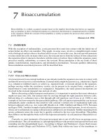
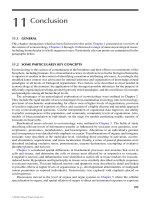
temperature) to limit primary production in terrestrial and aquatic ecosystems. Melillo et al. (1993)
used aterrestrial ecosystemmodel (TEM)to predictthe effects ofclimate changeand elevated CO
2

on
NPP. Spatially referenced information on climate, soils, vegetation, water availability, and elevation
were used to predict current NPPvalues fora widevariety ofecosystems. Model predictionsof current
NPP were very close to values based on field measurements. The model was then run to simulate
responses of NPP to a doubling of CO
2
and associated changes in temperature, precipitation, and
cloud cover as predicted by general circulation models (Figure 30.1). Overall global NPP increased
by approximately 23%, but there was considerable variation among ecosystems. This geographic
variation reflects not only how different ecosystems will respond to climate change but also the
underlying mechanisms. For example, moist temperate ecosystems responded primarily to elevated
temperature and increased nitrogen cycling whereas dry temperate ecosystems responded primarily
to elevated levels of CO
2
.
30.2.1.4 Global Patterns of Productivity
Productivity is not evenly distributed among regions of the world, and comparisons of NPP and
biomass estimated by Whittaker and Likens (1973) for some of the world’s major biomes reveal
Ecosystem type
Alpine tundra
Short grassland
Desert
Boreal forest
Temp. conif.
Temp. decid.
Temp. savan.
Trop. savan.
Trop. decid.
0
1

2
3
4
5
6
7
Current NPP
Predicted NPP
NPP (10
15
gC/y)
FIGURE 30.1 Results from a TEM used to predict the effects of a 2×increase in CO
2
and associated changes
in temperature, precipitation, and cloud cover on NPP of different terrestrial ecosystems. (Data from Table 2 in
Melillo et al. (1993).)
© 2008 by Taylor & Francis Group, LLC
Clements: “3357_c030” — 2007/11/9 — 18:39 — page 640 — #6
640 Ecotoxicology: A Comprehensive Treatment
TABLE 30.1
Estimates of Net Primary Productivity and Bio-
mass in the Earth’s Major Biomes
NPP (g/m
2
/y
2
) Biomass (kg/m
2
)
Terrestrial ecosystems

Tropical forest 1800 42
Temperate forest 1250 32
Boreal forest 800 20
Temperate grassland 500 1.5
Alpine and tundra 140 0.6
Desert scrub 70 0.7
Aquatic ecosystems
Algal beds and reefs 2000 2
Estuaries 1800 1
Lakes and streams 500 0.02
Continental shelf 360 0.01
Open ocean 125 0.003
Source: Data from Whittaker and Likens (1973).
several interesting patterns (Table 30.1). Although sunlight is necessary for primary production, it
is evident from Table 30.1 that other factors contribute to global patterns. If adequate moisture or
nutrients are not available, as in arid ecosystems or the open ocean, NPP will be low regardless of
the levels of sunlight. In forest ecosystems, a general decrease in NPP is seen as we move to colder
and more arid climates. The combination of sufficient sunlight, warm temperature, and abundant
moisture results in very high productivity for tropical forests. Despite the generally low productivity
of open ocean ecosystems, estuaries, algal beds, and coral reefs are among the most productive
aquatic habitats.
Biomass also varies among these different habitats and reflects different growth forms of the
major primary producers. Biomass in terrestrial habitats is generally much greater than in aquatic
ecosystems, and this large terrestrial biomass represents an important pool of global carbon. The
lower biomass in aquatic environments results from the relatively small body size of dominant
primary producers (e.g., phytoplankton), which has important implications for trophic dynamics.
Because small primary producers in aquatic ecosystems are capable of very rapid turnover, they can
support a relatively large biomass of consumers compared to terrestrial ecosystems. The ratio of
productivity to biomass (P:B) also varies greatly among different biomes and ecosystems. As shown
in Table 30.1, P:B ratios for terrestrial ecosystems, especially forests, are relatively low, reflecting

the large amount of nonphotosynthetic biomass in these ecosystems (e.g., bark, trunk, and branches).
In contrast, P:B ratios in aquatic ecosystems, especially those dominated by phytoplankton, are much
higher because of their small size and rapid turnover rates. The production values of lentic and marine
phytoplankton reflect multiple and overlapping generations, but biomass is measured at a specific
point in time. These differences in growth forms and turnover rates between terrestrial and aquatic
ecosystems may also have important consequences for responses to anthropogenic disturbances.
Because of their rapid growth rates, we expect that primary producers in aquatic ecosystems would
respond more rapidly to contaminants than in terrestrial ecosystems.
30.2.2 SECONDARY PRODUCTION
Secondary production is defined as the rate of productivity of consumers such as herbivores and
predators that obtain their energy from plant or animal biomass. Consumers such as bacteria and
© 2008 by Taylor & Francis Group, LLC
Clements: “3357_c030” — 2007/11/9 — 18:39 — page 641 — #7
Overview of Ecosystem Processes 641
TABLE 30.2
Measures and Definitions of Ecosystem Energetics and Efficiencies
Measure Definition
Consumption (C) Total amount of energy consumed
Egestion (E) Total amount of energy lost to egestion
Assimilation (C–E) Total amount of energy available for production and
respiration
Production (C–A) Total amount of energy available for growth and
reproduction
Assimilation efficiency (A/C ×100%) Portion of consumed food that is assimilated
Net production efficiency (P/A ×100%) Portion of assimilated food that is converted to new biomass
Gross production efficiency (P/C ×100%) Portion of consumed food that is converted to new biomass
Trophic level efficiency (A
n
/A
n−1

×100%) Efficiency of transfer of assimilated energy between two
trophic levels n, a consumer, and n −1, the resource
fungi, organisms that obtain energy from decomposing plant and animal material, should also be
included in measures of secondary production. Secondary productivity is similar to primary pro-
ductivity in that we must distinguish between the portion of energy for growth and reproduction
(and thus available to higher trophic levels) and the portion associated with maintenance costs of the
consumer (Table 30.2). As noted above, the amount of energy available to consumers is ultimately
determined by NPP and the efficiency with which fixed energy is converted to biomass. Similar to
the bioenergetic approaches described for populations, ecosystem ecologists have identified several
processes that limit efficiency of secondary production. Only a portion of the biomass consumed by
herbivores or predators is actually assimilated. Because food quality for predators is generally greater
than herbivores (i.e., proteins vs. recalcitrant cellulose and lignin), assimilation efficiency, which is
defined as the fraction of consumed biomass that is assimilated (e.g., available for growth, reproduc-
tion, respiration, and maintenance), is generally greater in predators. In addition to the recalcitrant
materials in plant tissue, herbivores must also contend with a diverse assortment of defensive chem-
icals produced by plants, which also limits consumption. Interestingly, coevolutionary responses
to these natural defensive chemicals may also explain the well-developed detoxification systems
in herbivores, which coincidentally provide protection against some xenobiotics. In contrast to ter-
restrial herbivores, assimilation efficiency is relatively high for zooplankton and other herbivores
feeding on unprotected phytoplankton or algae.
30.2.2.1 Ecological Efficiencies
Only a small fraction of the assimilated energy in consumers is available for growth and reproduction;
the remaining is necessary for maintenance and respiration. Because metabolic costs are generally
greater in homeotherms than in poikilotherms, net production efficiency, defined as the amount
of assimilated food available for new biomass, is generally lower in “warm-blooded” organisms
(1–2%) than in “cold-blooded” organisms (5–10%). Gross production efficiency, defined as the
amount of consumed food available for biomass, is a function of both assimilation and production
efficiencies. Finally, trophic level efficiency (also called Lindeman’s efficiency) is the efficiency of
energy transfer between two trophic levels. Although trophic level efficiency averages around 10%,
there is considerable variation among ecosystems (Pauly and Christensen 1995). The important

point is not the universality of the figure but the relative inefficiency of ecological systems. The
inefficiency of energy transfer also limits food chain length and the number of trophic levels in
an ecosystem (Table 30.3). Ricklefs (1990) estimated the average length of food chains based on
NPP, ecological efficiency, and energy flux of top predators for several different ecosystems using
© 2008 by Taylor & Francis Group, LLC
Clements: “3357_c030” — 2007/11/9 — 18:39 — page 642 — #8
642 Ecotoxicology: A Comprehensive Treatment
TABLE 30.3
Comparison of Average NPP, Predator Ingestion Rates, Ecological Effi-
ciencies, and Number of Trophic Levels in Marine and Terrestrial
Ecosystems
Community Type
NPP
(kcal/m
2
/y
2
)
Predator Ingestion
(kcal/m
2
/y
2
)
Ecological
Efficiency (%)
Number of
Trophic
Levels
Open ocean 500 0.1 25 7.1

Coastal marine 8000 10.0 20 5.1
Temperate grassland 2000 1.0 10 4.3
Tropical forest 8000 10.0 5 3.2
Source: Data from Ricklefs (1990).
the following equations:
E(n) = NPP Eff
n−1
(30.7)
n = 1 +
log[E(n)]−log(NPP)
log(Eff)
(30.8)
where n = number of trophic levels, E(n) = energy available to a predator at a trophic level n,
and Eff = geometric mean of the ecological efficiencies of transfer between each level. Results
showed that the number of trophic levels was more closely related to ecological efficiency than
overall NPP.
30.2.2.2 Techniques for Estimating Secondary Production
Estimates of secondary production for some species can be derived from measures of feeding rates,
assimilation efficiencies, and respiration in the laboratory (Fitzpatrick 1973) or under controlled
conditions (West 1968). However, determining secondary production in natural populations is more
challenging and generally requires estimates of consumption, growth, and reproduction. Sophist-
icated bioenergetics models have been developed for some aquatic species such as large-mouth
bass (Kitchell 1983). These individual-based models generally use laboratory-derived estimates of
consumption, respiration and elimination, and then solve for growth.
Consumption = Respiration +Wastes +Growth (30.9)
Several practical issues complicate our ability to estimate whole ecosystem production using these
individual-based models. While estimates of secondary production for individual species, especially
those for which we have a thorough understanding of natural history (Jordan et al. 1971, Kilgore and
Armitage 1978), have been developed, integrating this information to derive secondary production
estimates for whole ecosystems or even major components of ecosystems is challenging. Wiens

(1973) estimated secondary production of grassland bird communities, and Chew and Chew (1970)
examined energy relationships of dominant mammals in a desert shrub community. Perhaps the best
examples have been developed in aquatic ecosystems where researchers have derived community-
level estimates of secondary production for major taxonomic or functional feeding groups (Benke
and Wallace 1980, 1997, Carlisle 2000, Fisher and Gray 1983). Secondary production (P) in benthic
macroinvertebrates is obtained from estimates of biomass and growth rate using the following
© 2008 by Taylor & Francis Group, LLC
Clements: “3357_c030” — 2007/11/9 — 18:39 — page 643 — #9
Overview of Ecosystem Processes 643
simple relationship:
P = B
i
×g
i
(30.10)
where B
i
and g
i
are biomass and growth rates of the ith species.
While the methodology for estimating secondary production in aquatic ecosystems is well estab-
lished, these are labor-intensive efforts. Estimating biomass for macroinvertebrates is relatively
straightforward; however, the intensive sampling frequency necessary to determine growth rates
of macroinvertebrates often limits application of this technique. Because of these methodological
challenges, with few exceptions, secondary production has not received significant attention in the
ecotoxicological literature.An example of one such exception, Carlisle (2000) constructed food webs
based on quantitative analyses of macroinvertebrate secondary production for six different streams
along a gradient of heavy metal pollution.
Difficulties quantifying the role of detritus and the imprecise assignment of organisms to different
trophic groups are also impediments to studies of secondary production. Early attempts to quantify

the relationship between NPP and secondary production should be evaluated cautiously because of
the failure to appreciate the dominant role of decomposers and microbial production. The opinion
of O’Neill et al. (1986) that “the trophic level concept is most useful as a heuristic device and tends
to obscure, rather than illuminate, organizational principles of ecosystems” is likely shared by many
ecosystem ecologists. The use of stable isotopes, described in Section 34.4.4, is one potential solution
to this problem; however, relatively few studies have employed this technique in ecosystem-level
studies of secondary production.
30.2.3 THE RELATIONSHIP BETWEEN PRIMARY AND SECONDARY
PRODUCTION
Numerous studies have reported a direct quantitative relationship between primary productivity and
secondary productivity or biomass of consumers (Coe et al. 1976, Cyr and Pace 1993, McNaughton
et al. 1989). A major emphasis of the International Biological Program described in Chapter 29 was
to understand the biological basis of productivity and to quantify relationships between primary and
secondary production. Much of this research focused on understanding the underlying mechanisms
and consequences of interactions between plants and consumers. Some of the strongest evidence
to support the relationship between NPP and secondary production has been obtained from exper-
imental introductions of nutrients to whole ecosystems. The predictable increases in both primary
and secondary production illustrate the need to consider energy flow and nutrient cycling together
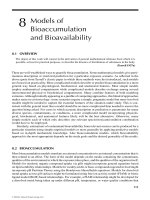
when investigating ecosystem energetics. Intuitively, we would expect that herbivore biomass or
production would increase with NPP; however, the nature of this relationship will likely vary among
ecosystems and herbivore types. For example, because grassland herbivores consume a larger por-
tion of NPP than forest herbivores (Whittaker 1975), the relationship between NPP and herbivore
abundance in forest ecosystems is relatively weak (Figure 30.2). Concentrations of structural com-
pounds, such as lignins and other recalcitrant materials that limit herbivory in terrestrial ecosystems,
are generally lower in aquatic primary producers. Consequently, grazers in many aquatic ecosystems
consume a large fraction of available biomass (30%–40%) and the relationship between primary and
secondary production in these systems is generally much stronger. Because a greater fraction of NPP
is removed in aquatic ecosystems, we also predict that predators would play a more important role
in energy flow here than in terrestrial ecosystems (Cebrian and Lartigue 2004). These expectations
are supported by studies showing the relative importance of top-down effects in aquatic ecosys-

tems compared to terrestrial ecosystems (Strong 1992). Predator control over lower trophic levels,
termed trophic cascades, has been frequently observed in aquatic ecosystems but only rarely in ter-
restrial ecosystems. Similarly, bottom-up control of herbivores and other consumers by nutrients and
primary producers is quite common in many lentic ecosystems and is the mechanism responsible
© 2008 by Taylor & Francis Group, LLC
Clements: “3357_c030” — 2007/11/9 — 18:39 — page 644 — #10
644 Ecotoxicology: A Comprehensive Treatment
Primary productivity
Secondary productivity
Forest ecosystems
Grassland ecosystems
Aquatic ecosystems
FIGURE 30.2 Hypothetical relationship between net primary productivity (NPP) and secondary productivity
in aquatic and terrestrial ecosystems. Stronger relationships are expected in aquatic ecosystems because grazers
consume a larger portion of plant biomass compared to terrestrial ecosystems.
for cultural eutrophication. Understanding the relationship between NPP and secondary production
in ecosystems is important for predicting potential contaminant effects. It is possible that some of
the variation in this relationship may account for differences in contaminant transfer rates among
ecosystems. These issues will be explored in Chapter 34.
30.2.4 THE RIVER CONTINUUM CONCEPT
The movement of materials and energy in ecosystems has been investigated using a variety of
descriptive, theoretical, and empirical approaches. Attempts to develop comprehensive explanatory
models that connect physical, chemical, and biological processes have been especially successful in
aquatic ecosystems. Vannote’s classic paper “The river continuum concept” (Vannote et al. 1980)
recognized that patterns and processes in streams change predictably from headwaters to the mouth.
In addition to linking geomorphologic characteristics of a watershed to biological processes, this
paper elucidated mechanisms responsible for the downstream transport, utilization, and storage of
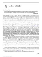
energy and materials. The major tenets of the river continuum concept (RCC) can be summarized by
considering longitudinalchanges inthe sourcesof energy andmaterials fromupstream todownstream
(Figure 30.3). The relative importance of allochthonous and autochthonous sources of energy shift

from upstream to downstream, resulting in changes in the ratio of NPP to respiration and structural
alterations in the composition of stream communities. Shaded headwater streams are generally
heterotrophic (P/R<1) because the dense riparian canopy in these systems limits primary productivity
and contributes significant amounts of allochthonous materials. Further downstream, as the canopy
opens, shading and the relative input of organic materials from riparian areas is reduced, and the
stream becomes autotrophic (P/R>1). Finally, large rivers may return to heterotrophic conditions
(P/R<1) because of increased depth and greater light attenuation.
Longitudinal changes in the abundance and composition of macroinvertebrate functional feeding
groups (Cummins 1973) along the river continuum are hypothesized to reflect the relative import-
ance of allochthonous and autochthonous inputs. The abundance of organisms that utilize coarse
particulate organic material (CPOM) (e.g., leaf litter) is greatest in headwater streams and decreases
downstream. Grazers, organisms that consume attached algae and periphyton, are more important
in mid-order streams where light levels are highest. Finally, organisms that collect fine particulate
organicmaterial (FPOM), includingcollector-gatherersand collector-filterers, dominate larger rivers.
Tests of thepredictions of the RCC indifferent geographicregions have provided good supportfor
the major tenets in NorthAmerica (Bott et al. 1985, Minshall et al. 1983) and Europe (Fleituch 1999).
Minshall et al. (1983) measured benthic organic matter, community metabolism, decomposition,
© 2008 by Taylor & Francis Group, LLC
Clements: “3357_c030” — 2007/11/9 — 18:39 — page 645 — #11
Overview of Ecosystem Processes 645
FPOM
CPOM
Shredders
Collectors
Predators
Grazers
Shredders
Collectors
Predators
Grazers

Collectors
Predators
1
2
3
4
5
6
7
8
9
Stream order
P > R
P < R
P < R
FIGURE 30.3 Major predictions of the river continuum concept showing changes in ecosystem energetics and
abundance of major functional feeding groups along a longitudinal stream gradient. (Modified from Figure 1
in Vannote et al. (1980).)
and functional feeding group composition along longitudinal gradients in streams from four distinct
geographic areas in North America. Although regional and local variation was observed, changes in
structure and function from headwaters to downstream sites were consistent with predictions of the
RCC. The RCC provided a unified theory describing structural and functional organization in stream
ecosystems that clearly illustrated the important connections between upstream and downstream
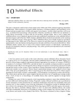
processes. Because of difficulty defining the spatial extent of stream ecosystems, streams of different
size within the same drainage had previously been treated as completely different systems. By
visualizing streams as a continuum of processes along a longitudinal gradient, ecologists recognized
that ecosystem function occurring in small headwater streams or large rivers could be described
using similar models (Figure 30.4). Despite differences in community composition and the relative
importance of allochthonous and autochthonous inputs, similar processes operate in both headwater
and mid-order streams. The RCC provided a conceptual framework for testing hypotheses about

factors that regulate stream ecosystem dynamics and radically modified the way that ecologists
visualized these systems.
30.3 NUTRIENT CYCLING AND MATERIALS FLOW
THROUGH ECOSYSTEMS
In Chapter 29, we defined ecosystem ecology as the study of the movement of energy and materials
through biotic and abiotic compartments of ecosystems. Figure 30.5 is a simple model illustrating the
connection between biotic and abiotic compartments and the processes that influence the movement
of materials through these compartments. Nutrients and other materials are assimilated from soil
or water by autotrophic organisms (plants and autotrophic bacteria), passed on to consumers, and
released back to abiotic compartments. The amount and availability of nutrients are among the most
important factors that limit primary productivity. In addition to limiting growth rates of primary pro-
ducers and heterotrophic microbes, nutrient availability also influences decomposition rates. The rate
of nutrient cycling may also influence ecosystem resistance and the rate of recovery from natural
© 2008 by Taylor & Francis Group, LLC
Clements: “3357_c030” — 2007/11/9 — 18:39 — page 646 — #12
646 Ecotoxicology: A Comprehensive Treatment
CPOM
Shredders
FPOM
Collectors
Primary
production
Grazers
Headwater stream
Grazers
CPOM
Collectors
Primary
production
Grazers

Mid
CPOM
Shredders
FPOM
Mid-order stream
FIGURE 30.4 Energy pathways and the importance of allochthonous and autochthonous materials in head-
water and mid-order streams. Despite considerable variation in the sources of energy and dominant functional
feeding groups, similar models can be used to characterize ecosystem dynamics. (Modified from Figure 1 in
Minshall et al. (1983).)
Animals
Primary producers
Bacteria
Detritus
Atmosphere
Soil
Water
Sediments
Photosynthesis
and assimilation
Organic compounds
(peat, coal, oil)
Inorganic compounds
(e.g., limestone)
Weathering
Erosion
Sedimentary
rock formation
Respiration
and excretion
Erosion, burning

fossil fuels
FIGURE 30.5 Simple model showing the connection between biotic and abiotic compartments and the dom-
inant processes that regulate movement of organic and inorganic materials among compartments. (Modified
from Figure 12.3 in Ricklefs (1990).)
and anthropogenic disturbances (DeAngelis et al. 1989). More importantly, an understanding of
nutrient and material cycles is essential for predicting ecosystem consequences of increased anthro-
pogenic inputs of certain materials, especially carbon, nitrogen, sulfur, and phosphorus. Predicting
the consequences of altered biogeochemical cycles also requires that we consider the ecosystem as
a unit instead of focusing only on component parts (O’Neill and Waide 1981). Because the behavior
and pathway of many toxic chemicals follow those of natural elements in ecosystems, considera-
tion of biogeochemical processes is essential for understanding fate and transport of contaminants.
© 2008 by Taylor & Francis Group, LLC
Clements: “3357_c030” — 2007/11/9 — 18:39 — page 647 — #13
Overview of Ecosystem Processes 647
Finally, we will see that many toxic chemicals have direct effects on ecosystems because they alter
biogeochemical processes.
30.3.1 ENERGY FLOW AND BIOGEOCHEMICAL CYCLES
The primary difference between movement of energy and nutrients through an ecosystem is that
nutrients are retained and constantly cycled between biotic and abiotic components by a variety of
meteorological, geological, and biological processes. In other words, the earth is considered an open
system with respect to energy but a closed system with respect to materials. Energy fixed by primary
producers is constantly supplied from an outside source and flows through the system. In contrast,
nutrients such as C, N, and P are assimilated, transformed, and released back to the ecosystem,
often in a very different form, where they can be used again. Meteorological processes include
precipitation, snowmelt, and atmospheric deposition. The major geological process is weathering
of materials from soils and underlying geological formations. Biological processes are analogous
to those discussed for energy flow and include transfers and transformations that occur within food
chains. If input of materials exceeds output, these unused materials may also accumulate in nutrient
pools, and their rate of movement between different pools is called the flux rate. If a nutrient pool size
is relatively constant, we can calculate the length of time an average molecule resides in this pool.

Residence time is calculated as the pool volume divided by the outflow of materials and is a good
measure of the accessibility of materials to organisms. For example, the atmosphere is a relatively
active pool for oxygen, with a residence time of about 20,000 years. In contrast, the atmosphere is
a storage pool for nitrogen, with a residence time of about 20 million years, reflecting the limited
accessibility of atmospheric N to organisms.
At a local level, if we assume that nutrient concentrations within a compartment are at equilibrium
(e.g., uptake is approximately equal to export), then measurement of uptake or loss provides an
estimate of turnover time within a compartment (Figure 30.6). Turnover time of organic materials and
nutrients variesamong ecosystemsand isclosely relatedto climateand temperature. Table 30.4 shows
the accumulation and mean turnover times for organic material and nitrogen in several different forest
types located in different climatic zones. Nitrogen and organic matter accumulations are greatest in
temperate coniferous forests, reflecting low rates of decomposition and efficient use of nutrients.
The low rates of decomposition observed in cold boreal forests result in a larger fraction of organic
material in soils relative to trees. Turnover time, the average amount of time that a molecule remains
in soil before it is assimilated by plants, increases in colder climates and is longer in coniferous
forests because foliage is not replaced each year.
Nutrient Pool or
Standing Stock
Biomass
Nutrient Pool or
Standing Stock
Biomass
Production
or input
Production
or input
Yield
or output
Yield
or output

Fast turnover
Slow turnover
Nutrient pool or
standing stock
biomass
Nutrient pool or
standing stock
biomass
FIGURE 30.6 The relationship between nutrient input, output, and turnover time. (Modified from Figure 25.1
in Krebs (1994).)
© 2008 by Taylor & Francis Group, LLC
Clements: “3357_c030” — 2007/11/9 — 18:39 — page 648 — #14
648 Ecotoxicology: A Comprehensive Treatment
TABLE 30.4
Accumulation and Turnover Times of Organic Matter and Nitrogen
in Different Forest Types from Different Biomes
Forest Type
Organic Matter
(kg/ha)
Turnover Time
(y)
Nitrogen
(kg/ha)
Turnover Time
(y)
Boreal coniferous 226,000 353 3,250 230.0
Boreal deciduous 491,000 26 3,780 27.0
Temperate coniferous 618,000 17 7,300 17.9
Temperate deciduous 389,000 4 5,619 5.5
Source: Data from Cole and Rapp (1981).

Atmospheric CO
2
(640)
Dissolved total CO
2
(30,000)
Algae
(5)
Bacteria
(1,500)
Respiration
(50)
Animals
Bacteria,
fungi
Plants
(450)
Dead organic
material (700)
Limestone, dolomite (18,000,000) Coal, oil, and natural gas (25,000,000)
Assimilation
(50)
(35)
Exchange
(84)
Assimilation
(35)
Respiration
(35)
(25)

Animals
Volcanoes (2)
Deposition (<1)
Dissolution (<1)
Combustion (<1)
Sedimentation (<1)
Oceans
Land
FIGURE 30.7 The carbon cycle. Numbers in parentheses indicate the amount of C in each compartment and
moving between compartments. (Modified from Figure 12.6 in Ricklefs (1990).)
30.3.1.1 The Carbon Cycle
Despite fundamental differences between the movement of energy and materials, nutrients and
other elements in biogeochemical cycles are closely associated with primary production and often
follow the flow of energy. The best example is the carbon cycle, which is intimately connected to
ecosystem metabolism and secondary production (Figure 30.7). Energy stored in carbohydrates by
primary producers is ultimately released when these high energy compounds are oxidized to CO
2
by
consumers and decomposers. The movement of carbon among compartments integrates biological
processes such as assimilation and respiration with physical processes such as atmospheric-oceanic
exchange, dissolution, and sedimentation.Although significant amountsof dissolved CO
2
are present
in the oceans, the largest pools of carbon are deposited in sediments (limestone, dolomite) and stored
as fossil fuels. Carbon dioxide occurs in a relatively low concentration in the atmosphere. Autotrophic
organisms (primarily plants) assimilate CO
2
and incorporate it into organic matter by photosynthesis,
and a portion of the CO
2

is returned to the atmosphere by respiration.
© 2008 by Taylor & Francis Group, LLC
Clements: “3357_c030” — 2007/11/9 — 18:39 — page 649 — #15
Overview of Ecosystem Processes 649
These physical, chemical, and biological processes are closely integrated in aquatic ecosystems
through the carbonate–bicarbonate system. The CO
2
dissolved in water forms carbonic acid, which
readily disassociates to bicarbonate and carbonate ions in the following reactions:
CO
2
+H
2
O ↔ H
2
CO
3
(30.11)
H
2
CO
3
↔ H
+
+HCO
−
3
(30.12)
HCO
−

3
↔ H
+
+CO
−
3
(30.13)
Because these reactions are dependent on pH, the amount of calcium (which equilibrates with the
bicarbonate and carbonate ions), and metabolism, they illustrate the close connection between biotic
and abiotic components as well as the relationship between carbon flux and energy flow. For example,
removal of CO
2
by photosynthesis or addition of CO
2
by respiration will drive these reactions to the
left or right, respectively, thus influencing pH. Because the concentrations of H
+
and CO
−
3
in aquatic
ecosystems significantly influencethe bioavailability of some contaminants, especially heavymetals,
alterations in the carbonate–bicarbonate system have important toxicological implications.
30.3.1.2 Nitrogen, Phosphorus, and Sulfur Cycles
Phosphorus is a major limiting nutrient in aquatic ecosystems and primarily responsible for eutroph-
ication of many lakes and streams. The P cycle is relatively simple because the atmosphere plays a
relatively small role. Consequently, transport of P in ecosystems is primarily sedimentary and at a
local scale. The major source of P to ecosystems is from underlying rocks (Figure 30.8), and loss
from soils is usually balanced by releases of inorganic P from weathering. Plants assimilate phos-
phorus as phosphate (PO

3−
4
), and availability and rate of uptake are dependent on pH. Herbivores
Plant, animal
Tissue (organic N)
Atmospheric N
Ammonia,
nitrates
Ammonia,
Ammonium
Lightning
Denitrification
Nitrification
N fixation
Assimilation
Ammonification
Nitrogen cycle
Plant, animal
tissue (organic N)
Ammonia,
nitrates
Ammonia,
ammonium
Denitrification
Nitrification
Herbivores
Plants
Soils
Phosphorus cycle
Rocks

PO
4
Inorganic
P
Excretion, decomposition
Weathering
Herbivores
Plants
Soils
Rocks
FIGURE 30.8 The phosphorus and nitrogen cycles showing the major biotic and abiotic pathways.
© 2008 by Taylor & Francis Group, LLC
Clements: “3357_c030” — 2007/11/9 — 18:39 — page 650 — #16
650 Ecotoxicology: A Comprehensive Treatment
obtain all of their required P from consumption of plants, and P is returned to soil by excretion
and decomposition. Whittaker’s (1961) tracer study quantified the movement of
32
P in an aquatic
microcosm from primary producers (phytoplankton, periphyton) to zooplankton. This study is an
excellent demonstration of the intimate relationship between nutrient dynamics and energy flow
through an ecosystem. Similar to the situation for many contaminants, this study also demonstrated
that the ultimate fate of
32
P was sediments, which was shown to be a major reservoir of P in aquatic
ecosystems.
The N cycle is considerably more complex because it involves a major atmospheric compon-
ent and because N can exist in numerous oxidation states. Five basic processes drive the N cycle:
nitrogen fixation, nitrification, assimilation, ammonification, and denitrification (Figure 30.8). The
vast majority of N occurs in the atmosphere as molecular N
2

, a form that is unavailable to plants.
Nitrogen-fixing bacteria in soil (Rhizobium) and cyanobacteria (blue-green algae) in aquatic envir-
onments convert atmospheric N
2
to ammonia. Nitrification is the process by which ammonia (NH
3
)
is oxidized first to nitrites (NO
−
2
) and then to nitrates (NO
−
3
) by several different groups of bacteria,
including Nitrosomonas and Nitrobacter. Plants assimilate N primarily as nitrate, and N is released
back to soils through decomposition and ammonification. Under anoxic conditions, another group
of denitrifying bacteria (Pseudomonas) reduces nitrates and releases inorganic N back to the atmo-
sphere. On a global scale, nitrogen fixation is balanced by denitrification. Anthropogenic release of
N to the biosphere has doubled the global rate of N fixation (Vitousek et al. 1997). These increases
in global emissions of N have significant consequences for aquatic ecosystems, including eutroph-
ication, toxic algal blooms (Burkholder and Glasgow 1997), and the formation of anoxic conditions
in the Gulf of Mexico (Rabalais et al. 1998).
Compared with other biogeochemical cycles such as C, N, and P, anthropogenic alteration of
the global sulfur (S) cycle by combustion of fossil fuels has been extreme. Approximately 60% of
the global S emissions are anthropogenic, resulting in widespread acidification of terrestrial and
aquatic ecosystems (Likens et al. 1996). The influence of acidification on ecosystem processes will
be described in Section 35.2. The S cycle is also relatively complex because S can exist in several
oxidation states, and conversion among these different forms is dependent on different types of
bacteria. Sulfur in a sedimentary phase such as organic matter and rocks can be released by natural
processes such as weathering and erosion. The gaseous form of S (H

2
S) is released from volcanoes
and decomposition of organic material. Sulfur released to the environment either by natural or
anthropogenic processes is oxidized to sulfate (SO
2−
4
) and deposited. Sulfur dioxide released from
the combustion of fossil fuels is oxidized and converted to sulfuric acid (H
2
SO
4
).
30.3.2 N
UTRIENT SPIRALING IN STREAMS
Unlike the situation observed in mature, undisturbed forests where most nutrients are generally
retained, a fraction of nutrients and other materials are transported downstream in lotic ecosystems
either in dissolved or particulate forms. Instead of cycling as observed in terrestrial systems, the
movement of nutrients in lotic ecosystems is generally represented as a downstream spiral (Elwood
et al. 1983, Webster and Patten 1979). Spiraling length is defined as the average distance that
a molecule travels as it completes a cycle between organic and inorganic phases. The length of
the spiral reflects uptake and turnover and is dependent on a variety of biotic and abiotic factors
including the rate of microbial mineralization, stream temperature, stream velocity, the shape of the
stream channel, and the number of snags and other woody debris that reduce downstream transport.
Uptake length, defined as the distance that a molecule travels before sorption to particulate matter or
uptake by organisms, is an important characteristic of ecosystem function. Uptake length essentially
measures nutrient uptake efficiency and is a useful indicator of anthropogenic disturbance.
S
w
= F
w

/wU (30.14)
© 2008 by Taylor & Francis Group, LLC
Clements: “3357_c030” — 2007/11/9 — 18:39 — page 651 — #17
Overview of Ecosystem Processes 651
where S
w
= uptake length, F
w
= downstream nutrient flux in water, U = uptake rate of nutrients
from water, and w = average stream width. Uptake length generally increases with stream discharge
and decreases with temperature, the amount of riparian vegetation, and biomass of detritus and algae.
In relatively small streams, attached algae, fungi, bacteria, and periphyton are responsible for
most of the uptake of nutrients, which generally follows Michaelis–Menten kinetics. Some of these
materials may be released back to the water column, but a fraction enters benthic food chains through
grazing organisms. Nutrients and materials continue to spiral downstream in larger rivers, but as
stream size increases nutrient dynamics in these systems more closely resemble patterns observed
in lentic ecosystems. The same processes that determine retention and transport of nutrients have
also been hypothesized to influence fate of contaminants in streams (Stewart and Hill 1993). It is
well established that periphyton and attached algae are important sinks for contaminants in lotic
ecosystems, and highly persistent chemicals may spiral downstream as they move between biotic
and abiotic compartments.
30.3.3 NUTRIENT BUDGETS IN STREAMS
The relative importance of allochthonous inputs to stream energy budgets has been well established.
However, the contribution of these terrestrial inputs to nutrient dynamics has received considerably
less attention. Whole ecosystem nutrient budgets have been calculated for a few relatively small
watersheds. In one of the most comprehensive studies, Triska et al. (1984) measured inputs from
litterfall, subsurface flow, and nitrogen fixation to develop an annual nitrogen budget for a small
stream in the H.J. Andrews Experimental Forest, Oregon, USA. Most of the total annual nitrogen
input (15.25 g/m
2

) was from subsurface flow (11.06 g/m
2
), with biological inputs contributing an
additional 4.19 g/m
2
. Direct and indirect biologically derived inputs from litterfall, throughfall,
lateral movement, groundwater, and nitrogen-fixation accounted for over 90% of the total nitrogen
to the stream. Total input of nitrogen was 34% greater than output, indicating that the stream was
not operating at a steady state. The difference between input and output was primarily a result of
storage of nitrogen as particulate organic matter.
30.3.3.1 Case Study: Hubbard Brook Watershed
Constructing nutrient budgets for whole ecosystems requires that we identify and measure the
processes that control inputs and outputs. Researchers at Hubbard Brook Experimental Forest,
a deciduous forest located in the White Mountains of New Hampshire, USA, have developed mass
budgets for a variety of nutrients (Likens et al. 1970). Because the Hubbard Brook watershed is
underlain by relatively impermeable metamorphic bedrock, inputs and outputs could be quantified
by measuring stream discharge, precipitation, and concentrations of materials in precipitation and
stream water. Because terrestrial losses of nutrients were eventually released to streams, measures
of atmospheric input from precipitation and fluvial output from streams could be used to construct
mass budgets for the entire watershed (Table 30.5). With the exceptions of NH
+
4
and NO
−
3
, output
of materials exceeded input, reflecting the weathering and leaching from soils and underlying rock.
One of the most significant findings of the research was that flux of nutrients was relatively small
compared to the pools of materials. This result demonstrates that, in stable watersheds such as Hub-
bard Brook, the majority of nutrients are usually retained and recycled. The export of sulfur, derived

primarily from atmospheric sources, was an important exception to this pattern. The significance of
this result will be discussed in Section 35.2.
30.3.3.2 Nutrient Injection Studies
Experimental injection of nutrients and tracers is the most direct method to examine retention and
transport of nutrients in streams. The general approach is to add a small amount of a radioactive
© 2008 by Taylor & Francis Group, LLC
Clements: “3357_c030” — 2007/11/9 — 18:39 — page 652 — #18
652 Ecotoxicology: A Comprehensive Treatment
TABLE 30.5
Mean Annual (1963–1968) Nutrient Budgets in the Hubbard
Brook Experimental Forest, New Hampshire, USA (kg/ha/year)
NH
+
4
NO
−
3
SO
2−
4
K
+
Ca
2+
Mg
2+
Na
+
Input 2.7 16.3 38.3 1.1 2.6 0.7 1.5
Output 0.4 8.7 48.6 1.7 11.8 2.9 6.9

Net change 2.3 7.6 −10.3 −0.6 −9.2 −2.2 −5.4
Source: Data from Likens et al. (1970).
or stable isotope at one point, and measure concentrations at several points downstream. Triska
et al. (1989) reported that 29% of the N injected into a third-order forested stream in California was
retained, while the remaining portion was transported downstream. Despite uptake by autotrophs,
which was greatest during the day, nitrate concentrations increased downstream, indicating that the
stream reach was a source of dissolved N to benthic communities. Decreased respiration and tissue
C:N ratios downstream of the injection point indicated a biological response to N enrichment.
Although the preferred method to measure nutrient dynamics and uptake length in streams is to
use tracers (e.g.,
32
P,
15
N) that maintain ambient concentrations, because of expense and logistical
issues, short-term additions that increase ambient nutrient concentrations are becoming increasingly
common (Davis and Minshall 1999, Hall et al. 2002). Although this approach may be useful for com-
paring different streams, Mulholland et al. (2002) reported that uptake length was overestimated by
short-term nutrient addition experiments compared to tracer additions. Because the degree of overes-
timation was related to the level of nutrient addition, these authors concluded that nutrient additions
should be as low as possible, while maintaining the ability to accurately measure concentrations at
several locations downstream.
30.3.4 T
RANSPORT OF MATERIALS AND ENERGY AMONG
ECOSYSTEMS
Our attempts to place spatial boundaries on ecosystems are compromised by our recognition that
materials and energy readily move between ecosystems. Aquatic ecologists have long recognized the
important connections between upland riparian and stream ecosystems. The significance of alloch-
thonous detritus to streams from surrounding upland areas was first described by Hynes (1970)
and figured prominently in the development of the RCC (Vannote et al. 1980). Streams serve to
connect processes occurring in upland terrestrial systems to lakes and oceans (Fisher et al. 1998).

However, streams are not simply conduits for nutrients and other chemicals but significantly alter
the quality and quantity of transported materials through input, storage, and instream biogeochem-
ical processes. The boundaries of stream ecosystems were previously considered to extend only
a short distance into the riparian zone. However, stream ecologists now recognize the important
linkages between streams and upland ecosystems (Fausch et al. 2002). Rather than visualizing
stream ecosystems as longitudinal corridors, recent studies emphasize vertical and lateral connec-
tions between the stream and surrounding landscape. Fisher et al. (1998) extended the nutrient
spiraling concept to include processes that occur outside of the stream. They suggested that the
nested, concentric arrangement of subsystems within stream ecosystems (e.g., surface water, hypo-
rheic zone, and riparian zone) is analogous to a telescope, where the length of the telescoping
cylinders reflects the processing length of materials. The processing length is the linear distance
required to transform an amount of material in transport. Thus, because processing length increases
with disturbance, we would expect that impacted systems would have lower rates of materials
cycling.
© 2008 by Taylor & Francis Group, LLC
Clements: “3357_c030” — 2007/11/9 — 18:39 — page 653 — #19
Overview of Ecosystem Processes 653
Salmon carcasses
Primary
production
Secondary
production
Terrestrial
scavengers
Anadromous
salmon
Riparian
vegetation
Juvenile salmon
growth and survival

FIGURE 30.9 The influence of anadromous salmon on production in aquatic and terrestrial ecosystems.
Although wehave traditionallyconsidered the transport of nutrientsand othermaterials in streams
as a one-way process, in some instances nutrients exported downstream may be returned to head-
waters. Marine-derived nutrients from anadromous Pacific salmon contribute significant amounts of
organic matter and N when the salmon return to their natal streams to spawn (Figure 30.9). Because
many of these streams are naturally oligotrophic and have a heavy canopy that limits primary pro-
ductivity, these nutrient subsidies can be very important to ecosystem productivity. Studies using
stable isotopic tracers of
15
N and
15
C have quantified the amount of marine-derived N andC delivered
to streams and adjacent riparian habitats. Because salmon are enriched with heavier isotopes of N
and C, comparisons of primary producers, consumers, riparian vegetation, and wildlife in streams
with and without spawning salmon have revealed the importance of these subsidies. In addition to
stimulation of primary producers and bottom-up effects on higher trophic levels (Bilby et al. 1996,
Wipfli et al. 1998), nutrients and organic material from salmon carcasses increase productivity and
diversity of riparian vegetation, and provide up to 25% of the N to riparian plants and 30–90% of
the N to the diet of terrestrial scavengers (Naiman et al. 2002). Increased primary and secondary
productivity associated with salmon carcasses translated to greater growth rates and survival of
juveniles inhabiting these streams, providing a positive feedback for returning salmon (Bilby et al.
1996). Similarly, declines in the abundance and biomass of spawning salmon that return to their
natal streams have important consequences for the function of both aquatic and adjacent terrestrial
ecosystems. In addition to transporting marine-derived nutrients to headwater streams, anadromous
fish also transfer contaminants from the oceans to relatively pristine streams (Ewald et al. 1998).
Although there is little information on the effects of these marine-derived pollutants on headwater
communities, levels of contaminants in resident (nonmigratory) species may increase significantly
(Ewald et al. 1998).
30.3.5 CROSS-ECOSYSTEM COMPARISONS
The vast majority of studies investigating processes that control rates of material cycling have been

conducted in single ecosystems or in a single type of ecosystem. The primary factors that influence
the rates of material cycling and energy flow (e.g., temperature, precipitation, vegetation, underlying
geology, and disturbance regime) vary significantly among ecosystems and geographic locations.
Comparisons of nutrient cycles among different ecosystems (e.g., tropical vs. temperate forests; arid
vs. humid grasslands; headwater streams vs. large rivers), at different altitudes, and among different
geomorphological units improve our understanding of these regulating factors and provide insights
into underlying mechanisms. Comparative studies across ecosystems may also provide the best
© 2008 by Taylor & Francis Group, LLC
Clements: “3357_c030” — 2007/11/9 — 18:39 — page 654 — #20
654 Ecotoxicology: A Comprehensive Treatment
opportunity to develop generalized models about material transfer and energy flow (Essington and
Carpenter 2000). Cross-ecosystem comparisons are essentially an optimization problem, where the
suitability of controls decreases but the ability to make broad generalizations increases among highly
dissimilar ecosystems (Fisher and Grimm 1991).
30.3.5.1 Lotic Intersite Nitrogen Experiment
Anthropogenic activities have resulted in increased N loading to aquatic and terrestrial ecosys-
tems primarily from agricultural activities and fossil fuel combustion. Because some of the excess
N deposited in headwaters is transported downstream, an understanding of factors that control N
uptake and export is essential for predicting ecosystem effects at the watershed level. In a compre-
hensive analysis of nutrient dynamics and metabolism in streams, researchers have used nutrient
tracer experiments to measure ammonium uptake and retention in 11 streams ranging from the North
Slope of Alaska to Puerto Rico (Mulholland et al. 2001, 2002, Peterson et al. 2001, Webster et al.
2003). The Lotic Intersite Nitrogen Experiment (LINX) compared stream metabolism and N dynam-
ics in tropical, arid, temperate, and tundra streams. The goal of this large-scale comparative study
was to relate inter-biome variability in stream metabolism and nutrient uptake to physical, chem-
ical, and biological characteristics. Stream metabolism (i.e., autotrophic primary production, and
autotrophic and heterotrophic respiration) was measured using the upstream–downstream diurnal
dissolved oxygen technique. To measure ammonium uptake,
15
NH

4
was injected in each stream and
samples were collected at downstream sites to determine uptake length. Stream metabolism (GPP)
was closely related to PAR (400–700 nm) and P concentration (Mulholland et al. 2001). Comparison
of results across different biomes indicated that ammonium uptake length varied by approximately
two orders of magnitude (14–1350 m) and increased with stream discharge (Webster et al. 2003). In
shallow headwater streams with a higher surface-to-volume ratio, most of the uptake and removal
processes occurred through assimilation by benthic autotrophic and heterotrophic organisms and by
sorption to sediments (Peterson et al. 2001). Because a large fraction of N inputs to headwater streams
was retained, especially during periods of high productivity, these systems regulated downstream
transport to lakes, rivers, and estuaries and thereby may reduce eutrophication.
30.3.5.2 Comparison of Lakes and Streams
Comparative studies of lakes and streams provide an opportunity to assess factors that regulate move-
ment of materials in two different types of ecosystems that vary widely in their major hydrologic
characteristics. The unidirectional flow of water is the defining physical property of stream ecosys-
tems. In contrast, lakes generally have low flushing rates, and therefore movement of materials is
dominated by vertical exchanges between epilimnetic, metalimnetic, and hypolimnetic zones. The
relative importance of allochthonous and autochthonous input is also quite different in lakes and
streams. Because of these differences, approaches used by ecologists to quantify nutrient cycling in
lakes and streams are quite different. Lake ecologists typically quantify the influence of nutrients
on primary production, whereas stream ecologists are more concerned with uptake length. In lakes,
uptake of nutrients occurs primarily by phytoplankton and bacteria, whereas periphyton and attached
algae play more important roles in lotic ecosystems. Grazing by zooplankton and subsequent return
of nutrients to the water column via excretion and mortality can occur rapidly in lakes. The rate at
which nutrients are deposited to and released from sediments is dependent on lake size, the volume
of throughflow, and seasonal changes in water temperature.
Because of differences in the movement of materials in lakes and streams, and the different meth-
odological approaches, a common currency is necessary to compare factors that regulate nutrient
cycling in lentic and lotic ecosystems. In both lakes and streams, cycling of nutrients is a function
of uptake and export of dissolved and particulate materials (Figure 30.10). Essington and Carpenter

(2000) developed a conceptual model to compare the recycling ratio, defined as the number of times
© 2008 by Taylor & Francis Group, LLC
Clements: “3357_c030” — 2007/11/9 — 18:39 — page 655 — #21
Overview of Ecosystem Processes 655
Dissolved nutrient pool
Particulate nutrient pool
Uptake Release
Import
Export
Particulate
Dissolved
Particulate
Dissolved
FIGURE 30.10 Conceptual model showing the import and export of dissolved and particulate nutrients in
aquatic ecosystems. (Modified from Figure 1 in Essington and Carpenter (2000).)
that a nutrient molecule is used before it is exported from the system, in lakes and streams. The
recycling ratio is a dimensionless number calculated as the ratio of uptake rate (U, mass ×time
−1
)
to export rate (E, mass ×time
−1
). According to this model, mass-specific export rates of nutrients
in particulate form (primarily to sediments) will be greater in lakes, whereas export rates of dis-
solved materials will be greater in streams. Nutrient cycling in streams is controlled primarily by
the association of nutrients with particles and downstream transport. In lakes, nutrient cycling is
controlled by physical processes that reduce the rate of sedimentation and biological processes that
increase remineralization. Essington and Carpenter’s (2000) model also predicts that the effects of
consumers (grazers in streams; zooplankton in lakes) will be fundamentally different in lakes and
streams. Although the model was developed to compare nutrient cycling in lakes and streams, it can
be used to quantify the movement of contaminants through these systems. We would expect that

movement of contaminants in streams would be dominated by downstream export in the dissolved
phase, whereas movement in lakes would be dominated by sedimentation.
30.3.5.3 Comparisons of Aquatic and Terrestrial Ecosystems
Relatively few studies have compared ecosystem processes across terrestrial and aquatic ecosys-
tems. In a comprehensive analysis of >800 aquatic and terrestrial systems, Cebrian and Largitue
(2004) examined factors that controlled herbivory and decomposition rates. Although NPP varied
greatly within aquatic and terrestrial ecosystems, there was surprisingly little variation between these
ecosystem types when analyzed across all studies. Nutritional quality of primary producers was an
important predictor of the proportion of NPP consumed by herbivores in both aquatic and terrestrial
ecosystems, indicating the extent of top-down regulation of producer biomass. In contrast, while
the total consumption by herbivores (g C/m
2
/year) was correlated with NPP, it was unrelated to
nutritional quality.
30.3.6 ECOLOGICAL STOICHIOMETRY
Energy has been considered the universal currency for studying ecosystem processes for several
decades. Although the transfer of energy through aquatic and terrestrial foodwebs can reveal much
about how ecosystems operate, our understanding of this process remains somewhat incomplete.
Ecological stoichiometry improves on this single currency approach by using ratios of certain ele-
ments (C, N, and P) to characterize how composition of organisms and their prey affect nutrient
cycling, production, and energy flow. Ecological stoichiometry is defined as the balance of multiple
chemical substances in ecological interactions and processes (Sterner and Elser 2002). By compar-
ing elemental ratios in abiotic compartments, primary producers, and consumers, limiting elements
© 2008 by Taylor & Francis Group, LLC
Clements: “3357_c030” — 2007/11/9 — 18:39 — page 656 — #22
656 Ecotoxicology: A Comprehensive Treatment
can be identified and a better understanding of utilization efficiencies and nutrient cycling can be
obtained (Anderson and Boersma 2004). Ecological stoichiometry has been used to examine link-
ages between N and C cycles in terrestrial and aquatic ecosystems. The approach is based on the
concept that relative amounts of elements in different compartments can regulate nutrient cycling

and energy flow. For example, C:N and C:P ratios generally decrease with trophic level in both
aquatic and terrestrial ecosystems. Simple trophochemical diagrams (Sterner and Elser 2002) may
be used to depict relative amounts of elements in different trophic levels and compare spatial (among
ecosystem types) and temporal stoichiometric patterns (Figure 30.11).
The study of ecological stoichiometry is critically important to our understanding of anthropo-
genic alterations in global nutrient cycles. Anthropogenic increases in CO
2
, N, or P will significantly
modify C:N and C:P ratios, thereby influencing rates of mineralization, energy flow, and decompos-
ition. Analyses of global increases in these materials indicate that N and P are disproportionately
enriched relative to C, thus potentially disrupting natural stiochiometric ratios of these elements
(Table 30.6). Because N and P enrichment will likely influence nutrient use efficiency, models
describing CO
2
effects on primary productivity cannot be considered in isolation but should also
account for anthropogenic increases in other nutrients (Sterner and Elser 2002). Similarly, elevated
Concentration of P
Concentration of N
Algae
Bacteria
Fish
Z
Concentration of C
FIGURE 30.11 Simple trophochemical diagram used in ecological stoichiometry todepict relativeamounts of
elements in different trophic levels and to compare spatial (among ecosystem types) and temporal stoichiometric
patterns. (Modified from Figure 8.1 in Sterner and Elser (2002).)
TABLE 30.6
Estimates of Natural and Anthropogenic
Releases of Carbon, Nitrogen, and Phosphorus
to Global Biogeochemical Cycles (Billions of

Metric Tons per Year)
Source C N P
Natural 61 0.13 0.003
Anthropogenic 8 0.14 0.012
Percent increase from 13 108 400
anthropogenic sources
Source: From Falkowski, P., et al., Science, 290, 291–296, 2000.
© 2008 by Taylor & Francis Group, LLC
Clements: “3357_c030” — 2007/11/9 — 18:39 — page 657 — #23
Overview of Ecosystem Processes 657
CO
2
will likely produce leaf litter with greater C:N ratios, resulting in lower rates of mineralization
and decomposition.
At a more local level, enrichment of certain elements resulting from anthropogenic releases may
alter processesoccurring inecosystems. On thebasis ofan analysisof major ecosystem compartments
(detritus, producers, and consumers), Dodds et al. (2004) measured C:N ratios and N-specific uptake
rates in streams located in several biomes. The C:N ratios increased from consumers to primary
producers to detritus. These researchers also reported a significant inverse relationship between
C:N ratios and N-specific uptake. These findings have important implications for N export and
eutrophication of downstream systems. Although undisturbed headwater streams are highly retentive
of N, anthropogenic deposition of N to these watersheds will decrease C:N ratios and increase
N export downstream (Dodds et al. 2004).
30.4 DECOMPOSITION AND ORGANIC MATTER
PROCESSING
Decomposition is the process by which dead organic matter (detritus) is broken down to its com-
ponent parts. Decomposition is a critical characteristic of ecosystem function and has been shown
to vary among ecosystems and with levels of disturbance. Decomposition rates are determined
by a complex interplay of physical, chemical, and biological processes. Factors such as chemical
composition and nutritional quality of detritus, physicochemical characteristics of the habitat, and

the abundances of decomposers influence decomposition rates. Decomposing organic material may
be consumed by detritivores or further processed by bacteria and fungi, with CO
2
and inorganic
materials (e.g., NH
4
) as the end products. Organic material may be fragmented into smaller sizes
by physical processes and invertebrates, thereby increasing surface area of particles. The net res-
ult is the conversion of particulate organic materials to dissolved constituents and the transfer of
carbon to decomposers and detritivores. In terrestrial ecosystems, the most important macroinver-
tebrate decomposers include nematodes, insects, isopods, crustaceans, and oligochaetes. In aquatic
ecosystems, CPOM is processed by shredders (primarily aquatic insects) and converted to FPOM.
30.4.1 ALLOCHTHONOUS AND AUTOCHTHONOUS MATERIALS
Secondary production of some aquatic ecosystems, particularly canopied headwater streams, may be
heavily subsidized by inputs of allochthonous materials. In contrast to autochthonous energy derived
from macrophytes, periphyton, phytoplankton, and other primary producers, allochthonous energy
sources consist of organic materials and detritus derived from outside sources. Detritus-based food
webs are common in many marine and lotic ecosystems. The relative contribution of allochthonous
and autochthonous materials to secondary production is dependent on the dimensions and shape of
the stream or lake and will be described in Section 31.2.3.
Although the elemental composition of leaf litter varies significantly among leaf species, much
of the nutritional quality provided to detritivores is derived from bacteria and fungi that rapidly
colonize leaf surfaces during decomposition (Suberkropp and Klug 1976). High nutritional quality
of detritusis expectedto increase growth rates and metabolic activity of detritivores and decomposers,
thereby increasing the rate of decomposition. In general, nutritional quality of detritus, expressed
as concentrations of N and P, is greater in aquatic ecosystems than in terrestrial systems. The rate
of detrital production is also highly correlated with NPP in both aquatic and terrestrial ecosystems
(Cebrian and Lartigue 2004). Therefore, factors discussed earlier that influence NPP such as light
and nutrients also play a role in determining decomposition rates and the size of detritus pools.
Because the fraction of NPP consumed by herbivores is greater in aquatic than in terrestrial

ecosystems (Cyr and Pace 1993), the amount of carbon channeled to detritus is generally greater
in terrestrial systems. Nonetheless, detrital pathways dominate the flux of carbon and nutrients
© 2008 by Taylor & Francis Group, LLC
Clements: “3357_c030” — 2007/11/9 — 18:39 — page 658 — #24
658 Ecotoxicology: A Comprehensive Treatment
in most ecosystems, with greater than 50% of NPP going to decomposers (Cebrian and Lartigue
2004). The fate of this material and the relative importance of invertebrate detritivores and microbes
have received considerable attention in the ecological literature. Studies conducted in aquatic and
terrestrial ecosystems have quantified decomposition rates, usually expressed as rates of leaf litter
decay. Various approaches have been employed to assess the relative importance of physical pro-
cesses, macroinvertebrates, and microbial processes in litter decomposition. Computer simulations
were used to calculate an organic matter budget for a second-order stream at Coweeta Hydrolo-
gic Laboratory, North Carolina (Webster 1983). Results showed that macroinvertebrate shredders
were responsible for approximately 27% of the downstream transport of particulate organic mater-
ial. Elimination of macroinvertebrate shredders using the pesticide methoxychlor (discussed in
Section 23.4.1.2) from a stream in this same watershed resulted in significant changes in dynamics
of detritus (Wallace et al. 1982).
The most compelling evidence demonstrating the significance of detritus to a stream food web
comes from experimental studies that increased nutrient concentrations or eliminated terrestrial
inputs. Elwood et al. (1981)showed that nutrientenrichment ofasmall heterotrophicstreamincreased
decomposition rates, resulting in greater abundance of consumers and higher trophic levels. Wallace
et al. (1997) used an overhead canopy to eliminate leaf litter inputs to a small headwater stream for
3 years. Benthic organic matter was lower in the treated stream, resulting in significant reductions in
abundance and biomass of most major taxa and declines in overall secondary production. Predator
production also declined in streams where leaf litter was eliminated, demonstrating strong bottom-up
effects and important linkages between detritus and higher trophic levels.
30.4.2 METHODS FOR ASSESSING ORGANIC MATTER DYNAMICS
AND
DECOMPOSITION
Although the complex interactions that occur within ecosystems are grossly oversimplified in many

food web diagrams, measuring the outcome of decomposition is relatively straightforward. Changes
in mass (dry weight) or nutrient content of organic material over time is generally used as an indic-
ator of decomposition rates. Long term assessments of organic matter dynamics can be obtained in
terrestrial habitats by measuring changes in total soil organic carbon pools using combustion tech-
niques. However, these methods do not provide an estimate of carbon availability, which is often
independent of the amount of carbon stored in pools (Robertson and Paul 2000). Fractionation of
organic carbon into humic acids, fulvic acids, and other constituents may provide some insight into
the availability of carbon to microbial decomposers (McKnight 2001).
To measure decomposition rates, organic material such as leaf litter is placed in mesh bags in
the field and then collected over a period of time (usually a geometric sequence of dates) to evaluate
mass loss and nutrient changes. Leaf or litter materials are usually collected from representative
and relevant species in the ecosystem. The decomposition rate constant, k, is estimated from the
following equation:
X
t
= X
0
×e
−kt
(30.15)
where X
t
is the mass remaining at time t and X
0
is the initial mass. The (first-order) decomposition
rate constant (k) is the slope of the least squares regression of proportion mass remaining versus time.
The magnitude of k reflects the rate of decomposition and varies greatly among different leaf species
and different ecosystems (Figure 30.12). Mesh size of litter bags is often manipulated to exclude or
include certain macroinvertebrate groups andto discernthe relativeimportance of macroinvertebrates
and microbes in decomposition. Mass loss may be related to the abundance or biomass of detritivores

that colonized the bags during the exposure period. Because small mesh of litter bags may impede
aeration or water flow, or create unnatural conditions, results of this technique should be interpreted
cautiously. Leaf litter decomposition studies in terrestrial ecosystems are generally conducted over
© 2008 by Taylor & Francis Group, LLC
Clements: “3357_c030” — 2007/11/9 — 18:39 — page 659 — #25
Overview of Ecosystem Processes 659
Time (days)
Mass remaining (%)
Arctic tundra
k = 0.005
Semiarid grassland
k = 0.25
Tropical forest
k = 1.40
FIGURE 30.12 Hypothetical relationship between percent mass remaining and time in three ecosystems with
varying decomposition rates. k = the decomposition rate constant.
longer time periods (1–3 years) than in aquatic ecosystems (3–6 months). Because contaminants will
affect both microbial processes and abundance of macroinvertebrate decomposers, values of k are
expected to decrease in stressed ecosystems.
30.5 SUMMARY
Flow of energy, cycling of nutrients, and decomposition of litter are fundamental processes in all
ecosystems. A basic understanding of these processes and how they vary spatially and temporally
is necessary to predict how these systems may respond to anthropogenic stressors (Howarth, 1991).
Because the components of ecosystems (e.g., populations and communities) may respond quite dif-
ferently to anthropogenic disturbances, an ecosystem perspective is necessary to limit the likelihood
of ecological surprises described by Paine et al. (1998). Because pathways of energy flow and
biogeochemical cycles in ecosystems are intimately coupled with the movement of contaminants,
basic models developed by ecosystem ecologists may also help explain fate of xenobiotic chemicals.
Each of the processes we have discussed in this chapter is likely to be affected by physical or chemical
stressors to some degree. The relative sensitivity and variability of these responses compared with

more traditional population- and community-level endpoints will likely vary among stressors and
among ecosystem types. In the following two chapters we will consider descriptive and experimental
approaches that have examined effects of stressors on these ecosystem processes.
30.5.1 SUMMARY OF FOUNDATION CONCEPTS AND PARADIGMS
• The perspective that ecosystems are highly complex may explain the relative infrequency
with which ecosystem processes are measured in biological assessments.
• Before we can understand how ecosystems respond to contaminants and other anthropo-
genic perturbations, it is necessary to develop an appreciation for the ecosystem processes
that are most likely to be affected.
• In addition to viewing ecosystems within a hierarchical context, ecologists routinely
characterize ecosystems based on bioenergetic and biogeochemical processes.
• Flux of energy through an ecosystem is determined by the rate at which plants assimilate
energy by photosynthesis, the transfer of this energy to herbivores and other consumers,
and the efficiency of these conversions.
• The energy necessary for the conversion of CO
2
to a reduced state in carbohydrates is
provided by visible light, and the total amount of energy fixed by plants is referred to
as GPP.
© 2008 by Taylor & Francis Group, LLC