Land Use Change: Science, Policy and Management - Chapter 2 docx

17
2
Developing Spatially
Dependent Procedures
and Models for
Multicriteria
Decision Analysis
Place, Time, and
Decision Making Related
to Land Use Change
Michael J. Hill
CONTENTS
2.1 Introduction 17
2.2 Concept 19
2.3 Transformation Issues 19
2.4 Transformation Domains and Methods 21
2.5 Example Landscape Context—Australian Rangelands 23
2.5.1 Spatial Patterns and Relationships 25
2.5.2 Temporal Patterns and Inuences 26
2.5.3 Data and Information: Scale of Representation 29
2.5.4 Some Spatiotemporal Inputs to a Rangeland MCA 30
2.6 A Framework for a Multicomponent Analysis with MCA 32
2.7 Conclusions 33
2.8 Acknowledgments 37
References 37
2.1 INTRODUCTION
Land use change occurs within a space-time domain. Frameworks for assessing
appropriate land use and priorities for change must capture the complexity, reduce
© 2008 by Taylor & Francis Group, LLC
18 Land Use Change
dimensionality, summarize a hierarchy of main effects, transfer signals and patterns,

and transform information into the language of the political and economic domains,
1

yet retain the key dynamics, interactions, and subtleties. Spatial interaction, temporal
cycles, responses and trends, and changes in spatial patterns through time are impor
-
tant sources of information for condition, planning, and predictive assessments.
Spatially applied multicriteria analysis
2
enables diverse biophysical, economic, and
social variables to be mapped into a standardized ranking array; used as individual
indicators; combined to develop composite indexes based on objective and subjec
-
tive reasoning; and used to contrast and compare hazards, risks, suitability, and new
landscape compositions.
3,4,5,6
The multicriteria framework allows the combination of
multi- and interdisciplinarity.
7
The system denition depends upon the purpose of
the construct, scale of analysis, and set of dimensions, objectives, and criteria.
7
When mapping both quantitative and ordinal data into factor layers, retention of,
and access to, rationale and reasoning for inclusion and weighting or contribution
to composites is important for maintenance of the link between the outcome of the
analysis and the real or approximate data used as input. This particularly applies to
spatial and temporal information. Here it is important to know what the meaning of
a spatial or temporal metric might be when it is included among other data in devel
-
opment of an assessment to aid decision makers. The meaning has two components:

(1) the rst relates to the direct description of the metric such as the average patch
size of remnant vegetation within a particular analytical unit, or the amplitude of
the seasonal oscillation in greenness from a normalized difference vegetation index
(NDVI) prole; (2) the second relates to what the metric measures in terms of inu
-
ence on the target issue; for example, patch sizes greater than
x indicate a higher
water extraction to water recharge ratio, resulting in a lowering of the water table, or
an amplitude equal to
y indicates a 75% probability that the area is used for cereal
cropping and hence has no water extraction capacity in summer. In the context of
multicriteria analysis (MCA), assignment of meaning to spatial and temporal metrics
depends on project-based research, wherein a relationship is established between
some aspect of land use change or condition, or some derived property of an input
variable layer, and a metric that is robust and translatable from study to study. Intrin
-
sically, some metrics have more easily ascribed meaning than others—the meaning
-
fulness being inversely proportion to the degree of abstraction and extent of removal
from biophysical, economic, or social measures that are a directly related to the
manifestation of land use change.
There is a very wide array of potential analytical adjuncts to MCA.
8
These can
be summarized into several groups of methods: those for dealing with input uncer
-
tainty; those applied to weighting and ranking; models and decision support systems
(DSS) delivering highly processed and summarized derived layers into the analysis;
various cognitive and soft systems methods requiring transformation for use, or
perhaps sitting outside of the standard MCA; optimization approaches; and integrated

spatial DSS, participatory geographical information (GIS) and multiagent systems.
However, the quantication, metrication, and summary of spatial and temporal
signals and temporal change in spatial patterns represent a level of sophistication
and derivation that has yet to be fully explored. Recent experience with the devel
-
opment of simple scenario tools for assessing carbon outcomes from management
© 2008 by Taylor & Francis Group, LLC
Developing Spatially Dependent Procedures and Models 19
change in rangelands
9,10
has emphasized the importance of spatial gradients, inter-
actions and patterns, and temporal trends and transitions in response to anthropo
-
genic and environmental forcing. In this chapter, the Australian rangelands are used
as an example coupled human-environment system to examine the role that spatial
and temporal information can play in a multicriteria framework aimed at informing
policy and by denition requiring a substantial element of social context.
There is a large and long-standing literature base dealing with signal processing
11

and time series analysis
12,13,14
and merging methods across these two areas.
15
This
literature indicates how the properties of demographic, economic, social, and bio
-
physical point-based time series data can be captured. With spatially explicit time
series we are interested in how these properties can be meaningfully mapped into a
multicriteria analysis framework.

2.2 CONCEPT
The premise behind this chapter is that some form of multicriteria framework is use-
ful for exploration of complex coupled human environment systems and for informing
policy decision making. Integration of nonscientic knowledge is of key importance,
and the user perspective may be the ultimate criterion for evaluation.
16
A requirement
of this analysis is that it is simple and transparent to the client, stakeholder, partici
-
pant, and decision maker, but that it has the capability to capture complex spatial and
temporal interactions and trends that inuence the nature of both system behavior
and evolution and the consequences of decisions. In principle, it is necessary for
multicriteria frameworks to include measures of system dynamics—both spatial and
temporal. Therefore, the underlying theme in this chapter is the efcacy, efciency,
and information content of transformations of spatial and temporal trends, patterns,
and dynamics into standardized, indexed layers for use in spatial multicriteria
analysis. The ensuing discussion does not imply that multicriteria approaches are
either the only way or the best way to approach analysis for policy decision making
in coupled human environment systems. It is simply one approach that has proven to
be useful,
4,6,17,18
and it provides a context for discussion of the issue of transformation
of spatial and temporal signals out of a complex multidimensional response space
into standardized, unitless, ordinal scalars to assist in human problem exploration
and decision making.
2.3 TRANSFORMATION ISSUES
In terms of denition, transformation is taken to mean a method by which a more
complex spatial pattern or relationship, or temporal pattern or trend, is mapped into
one to many quantitative metrics that have some functional relationship or under
-

standable descriptive contribution that can be ranked in terms of the objective of
a multicriteria approach. This transformation can therefore be a simple regression
function wherein the slope is used as the metric, or it can be a set of partial metrics
that together provide a composite indicator capable of being ranked. Examples of
the latter might include several spatial patch metrics such as number, size, and edge
length or several curve metrics such as timings, amplitude, and area under the curve.
© 2008 by Taylor & Francis Group, LLC
20 Land Use Change
Sexton et al.
19
dene four dimensions of scale:
(a) Biological—from cell, organism, population, community, ecosystem, land
-
scape, biome to biosphere; with four useful levels: (1) genetic, (2) species,
(3) ecosystem, and (4) landscape.
(b) Temporal—different spans of time for different events and processes.
(c) Social—example scheme: (1) primary interaction—physical human contact
with ecosystem, (2) secondary interaction—emotional (laws, policies, regu-
lation, votes, plans, assessments, and so forth), (3) tertiary—indirect and
qualitative (values, interests, cultures, heritage, and so forth).
(d) Spatial—many hierarchies based on numerous attributes.
Possibly the greatest issue in transformation relates to scale-dependent effects.
This is particularly so in human environment interactions where geographical varia
-
tion in human behavior and biophysical factors at different scales interact.
20
This is
also particularly so when combining biophysical data with economic and social data
where pixels and polygons with discrete spatial properties must be combined with
individual behaviors and institutional arrangements that operate in a multivariate

pseudospatial sphere of inuence
21
and have nonequivalent descriptions.
7
For example,
a region may be bound by certain rules that govern the degree of economic support
for certain activities. The potential spatial dimensions are the region boundary, but the
effective spatial pattern inside the region is governed by a range of existing conditions,
human characteristics and behaviors, economic conditions, and biophysical limita
-
tions, some of which can be directly supplied as spatial data layers, and some of
which require a model of potential inuence or effect to create an index of likelihood
of adoption or compliance. It is possible to establish equivalence rules between bio
-
physical and social landscape elements using structural (e.g., species composition
and hydrological system versus population composition and transportation and com
-
munication infrastructure), functional (e.g., patch connectivity versus commuting),
and change-based (e.g., desertication versus urbanization)
22
approaches. It is also
possible to establish demographic scale equivalence between biophysical and social
domains using a spatial hierarchy based on individuals (e.g., plants and people),
landscapes (e.g., watersheds and counties), physiographic regions (e.g., ecoregion
and census region), and extended regions (e.g., biome and continent).
22
Relationships of information derived within one scale category are reliant
on assumptions from others.
19
In a more general sense, the modiable areal unit

problem (MAUP), where correlations between layers vary with different reporting
boundaries, requires excellent transformation methods, using ner scale data to
inform the broader scale analysis,
23
and constant awareness of the potential problem
of understanding and managing patterns, processes, relationships, and human actions
at several scales.
19
Multiagent simulation approaches
24
have considerable benets in
dealing with individual behaviors in urban and densely populated system problems
25

as well as land cover change problems
26
and technology diffusion and resource use
change.
27
They may also be applied to examine emergent properties at the macro-
scale from different microscale outcomes and incorporate spatial metrics.
28
The second major issue in transformation relates to a meaning or quantiable rela-
tionship with an attribute that affects or contributes to assessment of the objective
© 2008 by Taylor & Francis Group, LLC
Developing Spatially Dependent Procedures and Models 21
of the analysis. A key element here is the eldwork and analytical work to develop
specic and general quantitative, probabilistic, or qualitative relationships between
patterns and processes
29,30,31

that can be used either locally or globally to assign a rank
in terms of some multicriteria objective. Laney
32
describes two approaches: studies
identifying the land cover and change pattern, then seeking to develop a model to
explain these patterns (pattern-led analysis) and studies that develop a theory to guide
pattern characterization (process-led analysis). Both approaches may have aws, with
pattern-led analysis being highly data dependent and able to identify only processes
associated with that data, and process-led analysis dependent on the prior theoretical
model, adherence to which may preclude treatment of other equally valid processes and
paths. The ultimate integration of transformation and meaning might be represented
by the “syndrome” approach,
33
wherein alternative archetypal, dynamic, coevolution
patterns of civilization-nature interaction are dened (e.g., desertication syndrome).
These syndromes might be characterized by highly developed composite indicators
that incorporate complex derived spatiotemporal relationships and patterns.
2.4 TRANSFORMATION DOMAINS AND METHODS
The effectiveness of a multicriteria framework is probably proportional to the extent to
which system elements and interactions are captured. Representation of time in tradi
-
tional GIS platforms is very poor,
34
while image-processing systems that handle time
series of spatial data lack the tools for extraction and summary of information from the
time domain. More accessible space-time analytical functionality is needed to make a
wide variety of transformation approaches available to those other than expert spatial
analysts and signal processors. The challenge lies in acquiring data in all of the poten
-
tial response domains at a suitable scale and with acceptable quality. A list of possible

information domains is given in Table 2.1 along with the kind of transformation issue
involved and some possible methods. Where individuals are involved, demographic
information coupled with surveys and units of community aggregation form the basis
for transformation—spatially in terms of the location of behaviors and recorded pref
-
erences in relation to land use patterns and changes, and temporally in the sense that
trajectories in opinion and behavior lead to land use change. Social systems are reex
-
ively complex (i.e., having awareness and purpose). Therefore, within a social multi-
criteria analysis with nonequivalent observers and nonequivalent observations, there is
a need to dene importance for actors and relevance for the system.
7
The actors in social
networks that inuence the land use outcome must be spatially represented,
35
but there
is a challenge in capturing the link between inuence and biophysical outcome.
36
At the level of social and economic statistics, collection units often determine the
nature of the analysis. Social indicator data may be idiosyncratic at the local scale,
have incomplete time series, have denitional changes over time, and have misaligned
reporting boundaries.
37
This results in MAUP, ecological fallacy, expedient choice of
statistics, arbitrary choice of measures, and difculty in establishing any causal rela
-
tionships.
37,38
Transformations are required to summarize temporal trends and cycles
and to dene spatial patterns and relationships at a ner scale, which may help to

distribute the information downward from the collection unit in scale in a spatially
explicit way. Dasymetric mapping can be used only to assign populations to remotely
© 2008 by Taylor & Francis Group, LLC
22 Land Use Change
TABLE 2.1
Transformation Domains for Spatiotemporal Multicriteria Frameworks
Information Domain
Transformation Issue Methods
Individual behaviors and
preferences
Representation of individual at
resolution of analysis
Transform survey information into
statistics and metrics that
summarize the tendencies in the
population for that spatial unit
Individual perceptions Representation of abstract
concepts such as beauty, degree
of space contamination, etc.
Use landscape image metrics,
spatial distances and landscape
contents
Institutional arrangements,
government regulations,
and incentives
Representation of the inuence
or likelihood of adoption or
compliance
Develop probability models based
on prior surveys of impact and

create probability layers
Economic variables Relating collection unit to
analysis unit
Self-organization of spatial units;
temporal trends, metrics, and time
period summaries
Social statistics, societal
systems, transport and
surveys
Conversion to a factor layer—
attaching a meaning and a rank
Develop probability models and
partial regression models to
ascribe some of variation in target
issue to the social factors. Create
factor layers based on the
percentage variation described,
direction (+ or –) and strength
(slope) of trend
Climate Impact/response an outcome of
complex temporal sequences
and spatial patterns
Develop impact threshold and
severity layers based on multiple
scenario runs
Disturbances—re,
grazing, clearing,
ooding, desertication,
urbanization,
abandonment

Representation of spatial extent,
spatial gradient, timing,
duration, impact, agents (i.e.,
active units such as animals)
Derive metrics describing spatial
and temporal patterns, harmonics,
limits, responses, demographics
that can be ranked in terms of the
target issue
Land use Representation of persistence
and change at level of cover
type, species, management
practice, seasonal magnitude
Derive metrics that capture pattern,
change, persistence, sequence, and
all quantitative properties of the
change in a hierarchical structure
Bio/geochemical process—
hydrology, sedimentation,
nutrients, gas exchange,
emissions, consumption
Representation of process in
terms of outcome affecting or
inuencing target issue
Aggregated, averaged, summarized
and probability converted outputs
from process modeling
© 2008 by Taylor & Francis Group, LLC
Developing Spatially Dependent Procedures and Models 23
sensed urban classes, and population surfaces can be created by associating the count

with a centroid and distributing it according to a weighted distance function.
38,39
The
relationship between people and their environment is captured by cognitive appraisal
from perceived environmental quality indicators.
40
Indicators of residential quality
and neighborhood attachment
40
might be transformed into spatial properties by
assigning proximity functions to services, assigning distance metrics to road access
and access to green space, ranking buildings for aesthetics and quality of human
environment, and mapping these with spatially explicit viewability constraints.
Climate provides an overarching inuence that is both spatially generalized and
locally spatially dependent, and it is a fundamentally time-dependent and cyclical
factor. Here the transformations include spatial patterns of microclimatic variation
and temporal trends in climate change, metrics of seasonal cycles and trends, or vari
-
ance in extremes. The remaining information domains are the most spatially and tem
-
porally interactive, with biogeochemical processes interacting with land use type and
change highly inuenced by human and other disturbances. These domains require
many spatial and temporal metrics as well as higher level measures of system response
in the form of outputs of spatially and temporally explicit models (e.g., hydrology).
Some methods for transforming complex spatial and temporal patterns, relation-
ships, and signals are given in Table 2.2. These are considered in terms of the general
spatial context, the specic social network data where spatial and nonspatial cogni
-
tive domains mix,
40

the visual context where views and beauty perceptions inter-
mingle with functional and locational considerations,
41
and the temporal context
where methods from nonspatial time series analysis complement methods specically
developed for time series of satellite data. The spatial and temporal contexts are
discussed in more detail in the following sections; however, the example landscape
context used in the discussion must rst be described.
2.5 EXAMPLE LANDSCAPE CONTEXT—AUSTRALIAN RANGELANDS
The Australian rangelands provide a suitable combination of spatial and temporal
dynamics and dependencies for illustration of issues surrounding transformation
of spatial and temporal system properties into an MCA framework. This system is
characterized by a hierarchy of scales within and across which inuences, effects,
relationships, and functions operate. All of the scale domains of biological, temporal,
social, and spatial are relevant. The system is affected by very large-scale climate
and economic factors and very small-scale spatial dependencies in habitats and land
-
scape function. The rangelands have the following characteristics:
1. Diversity in climate, soils, and vegetation types (Figure 2.1).
2. Heavily utilized by domestic livestock.
3. Substantially infested with feral animals.
4. A signicant biomass and soil carbon reserve and a source of greenhouse

gas emissions through annual wildre.
5. System principally limited by water availability.
6. Spatial interactions, patterns, and gradients substantially related to landscape
scale terrain–water dynamics and anthropogenic water supply (bores).
© 2008 by Taylor & Francis Group, LLC
24 Land Use Change
7. Temporal dynamics heavily inuenced by interaction between climate

(water supply), grazing and re.
8. Meso-scale landscape properties strongly linked to overall landscape function,
particularly in relation to water harvesting and consequent habitat development.
9. Signicant social issues through indigenous rights and sacred sites and site-
based tourism.
10. Management of the landscape is inuenced by exogenous temporal varia
-
tion in cost of nance and inputs, trade barriers and restrictions, price of
commodities, specically beef cattle, and changes in family structures and
rural employment.
TABLE 2.2
Methods for Exploration and Transformation of Complex Spatial and
Temporal Patterns, Relationships, and Signals
Spatial
23
Convolution ltering (moving window or kernel) containing functions from simple statistics to
textural indexes to complex regression to spatial autocorrelation
Distance measures in spatial neighborhoods—association of patch, gap and shape with socioeconomic
change factors
29
Cost–distance generation of user and purpose dened analysis units
Geographically weighted regression
49
to overcome nonstationarity, spatial dependencies, and
nonlinear spatial distributions, allowing classication of system parameters by a learning
algorithm—self-organization
Spatial/social networks
35–50
Resilience, fast and slow adjustment, perturbation, catastrophe, turbulence, and chaos models
51

Bioecological models—analysis of dynamic phenomena of competition-complementarity-substitution
(network as a niche); social landscape analysis in landscape ecology
22
Neural networks—not easily interpretable from economic view
Evolutionary algorithms—genetic algorithms with binary strings; evolutionary algorithms with
continuous setting and oating point values
Visual
41
Characteristic features—lower-upper feature relationships; contour block drawings; image textures;
contours and horizon; spatial relations of spaces and elements; proportions of landscape zones in
view; hierarchical properties; typology of fringes
Spatial distance measures—view texture; intrusion into skyline and landscape line; relative structural
complexity; relative proportions; distance–size relationships
Sensitivity—functional distance in landscapes; structural distances to be kept free
Temporal
Traditional time series analysis
12,14,52,53
—trends, cycles, seasonality, lags, phase, irregularity,
smoothing, differencing, autocorrelations, spectral analysis
Curve metrics
43,54
—limits, amplitude, periodicity, timings, areas, slopes, trajectories
55
; phenology
Signal processing—Fourier transforms
56
; Wavelet transforms
15,44
Principal component analysis of time series
44

Complex bio-socioeconomic cycles (e.g., Kondratieff waves
57
); syndromes of change
33
© 2008 by Taylor & Francis Group, LLC
Developing Spatially Dependent Procedures and Models 25
The system represents a type of example where human demographics are not a
major factor since large pastoral leases are essentially unpopulated except for the
station homestead and associated buildings. Human inuence in this environment is
provided through management, which reaches out from the homestead to inuence
very large tracts of land. Hence, supercially it might be difcult to draw method
-
ological parallels with the many coupled human environment systems worldwide
and high human population densities. However, in this system, demographics are
still important since the major inuential population is that of domesticated beef
cattle, with ancillary inuence from feral animal populations. They are individual
economic units with costs associated with parasite and disease control and human
handling and value in terms of food and breeding potential. The decision-making
framework for cattle is much less complex than for humans; cattle require water,
feed, shade, and socialization and will optimize their behavior within this response
space. Nevertheless, they inuence and respond to spatial and temporal patterns,
and, therefore, this system can still provide useful methodological insights.
2.5.1 SPATIAL PATTERNS AND RELATIONSHIPS
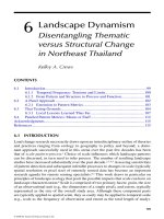
The spatial interrelationships in this rangeland system can be illustrated by a stylized
landscape containing articial water points surrounded by piospheres of inuence by
grazing animals upon the vegetation up to a distance limit (Figure 2.1). These water
points occur within fenced paddocks, parts of which are inaccessible to stock since
they are outside the water access limit. The paddocks also contain different land
cover types with different habitat suitability, re susceptibility, and livestock carrying
capacities. The landscape has rocky areas, areas with thick shrubland inaccessible to

stock, swampy and saline areas with low productivity, and an aboriginal sacred site.
The area also has an aesthetic component with a viewpoint and rest area located on a
major road, with basic picnic facilities outside the mapped extent. The major spatial
Water point piosphere of grazing intensit
y
Fenced paddocks
Heavily thickened woodland with shrubs
Poor, light soil
Inaccessible rocky outcrop
Swampy area with unpalatable plants
Saline scald area
Elevation contours
Sacred aboriginal site
FIGURE 2.1 The concept of grazing piospheres interacting with landscape structure to create
spatially and temporally dependent response zones in Australian rangelands. These are more
prevalent where rainfall is less reliable, paddocks are smaller, and stocking pressure is higher.
© 2008 by Taylor & Francis Group, LLC
26 Land Use Change
gradients in this landscape are created by the effect of grazing on vegetation and
habitat, the connectivity between habitats, the structure in relation to shelter, water
harvest and stock access, and the appearance of the landscape from a specic direc
-
tion and angle of view.
In order to capture spatial attributes, a level of spatial pattern reporting must be
dened, and this level of aggregation must be compatible with the resolution of other
data in the analysis. The scale of aggregation might relate to some functional distance
and sphere of inuence in the landscape, and pattern extraction might be undertaken
for a number of different aggregation units,
42
a nested set of patch scales,

30
in order
to specically capture the inuence of landscape structure from different elements
of the system such as bird habitat, cattle grazing behavior, scale of microtopography,
and so forth.
2.5.2 TEMPORAL PATTERNS AND INFLUENCES
The temporal behaviors of, and inuences on, this rangeland system could be
described by a time series of weather and satellite data, which records sequences
of detectable land cover change and vegetation state, as well as derived measures of
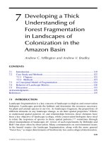
system function integrated through models. A monthly time series of net ecosystem
carbon exchange (Barrett, personal communication) provides an example data set
for illustration of approaches to disaggregation and decomposition of signals into
meaningful indexes (Figure 2.2). A series of seasonally based system responses pro
-
vide the basis for extraction of:
1. Curve metrics that describe the timing, duration, magnitude and periodicity
of the response
43
2. A cumulative aggregate of the net system behavior through time
3. Trend in signal from wavelet or other transforms
15,44
4. Temporal autocorrelation to see how strong the “memory” is in the system—
a strong memory indicates more regular cyclical behavior
5. Power spectrum and Fourier transforms on original data and rst differ
-
ences or rst derivatives to detect major cyclical patterns—in this case
occurring at about 22, 44, and 66 months
6. Cumulative probability curves to identify the relative behavior for some
proportion of cases (Figure 2.2)
These metrics and measures of time series attributes can be derived spatially and

converted to single or partial component indicators of system properties.
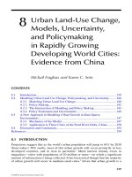
The temporal inuences are also represented by nonbiophysical time series such
as livestock numbers, climate cycle indexes, prices and costs, and human activity
measures (Figure 2.3). These data may only be available at a coarse level of spatial
resolution, such as cattle numbers from the agricultural census, or individual behaviors
from social surveys with limited samples. Alternatively, they may be global variables
such as cattle prices, interest rates, and climate indexes such as the southern oscilla
-
tion index (SOI). In these cases, a means must be found to apply these spatially via
some ltering layer that assigns the attributes only to those pixels where the inuence
occurs, or to those pixels not constrained by other factors.
© 2008 by Taylor & Francis Group, LLC
Developing Spatially Dependent Procedures and Models 27
–
2
0
–
4
0
–
0.02
0.00
0.02
–
0.4
0.0
0.4
0.8
0.0
0.2

–
0.2
0.0
0
40
80
NEP 1981
–
2000
NEP
Cumulative NE
P
Response
Signal
Autocorrelation
Power
Spectrum
Power
Spectrum
First
Difference
Cumulative
percentage
Normal score
Wavelet transform
Trend line
Fourier transform
Running cumulation
Time in months
Time intervals

Metrics
Amp
Integral
Interval
Period
0 12
T1 T2
4 8
Max
Min
0.5 Amp
0.2
0.0
0 24 48 72 96 120 144 168 192 216 240
0.00000
0.00008
0.00016
–
2
–
1 0 1 2 3 4
0.00000
0.00010
FIGURE 2.2 Time series approaches to extracting signal summary indicators. A time series
of net ecosystem productivity indicates the base potential for carbon xation. This may be trans-
formed into indicators by calculating metrics, including a running integral, extracting the fre-
quency of cyclic patterns using fast Fourier transform (FFT) or power spectrums on original data
or rst differences and derivatives, dening direction of temporal change through trend analysis
or wavelet transforms, and estimating likelihood of various levels though cumulative probability.
© 2008 by Taylor & Francis Group, LLC

28 Land Use Change
–
20
0
20
S
O
I
0
2
0
4
8
12
P
o
w
e
r
0
40
80
120
0
200
400
600
0
0
20

40
60
1976 1978 1980 1982 1984 1986 1988 1990 1992 1994 1996 1998 2000
2 4 6 8 10 12 14 16 18 20 22 24 26 28 30 32
1978 1980 1982 1984 1986 1988 1990 1992 1994 1996 1998 2000
1978 1980 1982 1984 1986 1988 1990 1992 1994 1996 1998 2000
1980 1982 1984 1986 1988 1990 1992 1994 1996 1998 2000
Cattle No. (million)
1976 1978 1980 1982 1984 1986 1988 1990 1992 1994 1996 1998 2000
8
9
10
11
12
Interest payments
Handling/marketing
Wages
–
hired hands
Age
–
owner
Age
–
spouse
Hours worked
–
owner
Hours worked
–

spouse
Cattle ($/head
)
Costs ($
)
40000
80000
120000
Age/Hour
s
IPO
FIGURE 2.3 Nonbiophysical time series also provide potential indicators but may not be
spatially explicit at the required scale. These need to be transformed into indicators such
as trends in demographics (e.g., cattle), patterns of climate and frequency of occurrence of
certain climate types, trends in prices for commodities, trends in costs of production, and
trends in human activities potentially affecting management and economic outcomes.
© 2008 by Taylor & Francis Group, LLC
Developing Spatially Dependent Procedures and Models 29
The spatial extent of discrete and consistent temporal patterns may be dened by,
for example, a principle components analysis (PCA) on the time series and subsequent
classication (Figure 2.4a). This reveals distinct temporal patterns that represent
a regional summary (Figure 2.4b; the temporal net ecosystem productivity (NEP)
signal for one of these classes is used in Figure 2.2). By contrast, time series attributes
may be calculated on a pixel-by-pixel basis, and the data, such as standard deviation
in NEP, are mapped to provide a continuous factor layer. The analysis of the trends in
the time series (Figure 2.2) may provide information about major periods of differing
behaviors, such as the net loss carbon throughout northern Australia between 1985
and 1993, versus the net gain in carbon between 1994 and 2000 (Figure 4.2c).
2.5.3 DATA AND INFORMATION: SCALE OF REPRESENTATION
Moving down scale to the region of interest for analysis, the Victoria River District

(VRD) in the northern Australian rangelands provides a good basis for assessment of
(a) (b)
(c) (d)
PCA classes
1
2
3
4
5
6
7
8
9
10
11
12
13
14
15
16
17
18
19
20
21
22
St. Dev. NEP
0.004
–
0.027

0.027
–
0.05
0.05
–
0.073
0.073
–
0.096
0.096
–
0.118
0.118
–
0.141
0.141
–
0.164
0.164
–
0.187
0.187
–
0.21
0.21
–
0.233
NEP 8593
<
–

2
–
2
–

–
1
–
1
––
0.5
–
0.5
– –
0.2
–
0.2
–
0
0
–
0.2
0.2
–
0.5
0.5
–
1
>
1

NEP 9400
<
–
2
–
2
–

–
1
–
1
––
0.5
–
0.5
– –
0.2
–
0.2
–
0
0
–
0.2
0.2
–
0.5
0.5
–

1
>
1
FIGURE 2.4 (See color insert following p. 132.) (a) The spatial pattern of temporal
signals may be grouped by applying principal components analysis to the time series and
creating a classication based on the major principal components. (b) The temporal metrics
may be calculated on the spatial times series to create maps of, for example, standard devia-
tion of net ecosystem productivity (NEP). (c) A running integration, trend, or wavelet analysis
may dene periods of distinct behavior in the time series that can then be summarized by
metrics such as an integral of NEP for periods of decline and increase. Shown for 1985–1993
and 1994–2000 here.
© 2008 by Taylor & Francis Group, LLC
30 Land Use Change
data scales and transformation through spatial ltering (Figure 2.5). The region has
three of the PCA classes given in Figure 2.4a. The temporal signal and associated
metrics and time series attributes could be broadly assigned to all areas within the
class zone in the VRD. However, the NEP data represent the response of the system
undisturbed by livestock. Therefore, in the absence of specic estimates that take the
spatially variable impact of grazing intensity around water points into account, one
could apply an arbitrary scaling of effect on NEP that varies from using the supplied
signals for ungrazed areas, to completely suppressing the accumulation signal at the
water point, where stock pressure is highest. Very broad scale estimates of prot per
hectare at full equity provide an indication of protability. Mine presence is indicated
by a count for each 1 km pixel—a decision may need to be made about a buffering
rule for radius of disturbance. The number of threatened birds is derived from a very
coarse resolution data set. However, if any information is available on the habitat
for these birds, then, for example, an index of potential threat to ground dwelling
birds could be created with very ne spatial resolution using a rule governing degree
of disturbance with distance from cattle watering points. Completely aspatial, but
important, system attributes and metrics may be downscaled to appropriate resolu

-
tion if relationships to spatial data at an appropriate resolution are known or can be
derived. The major challenge arises in ascribing causal relationships and areas of
interest to human population centers based on social statistics about activities and
preferences of humans. However, certain key variables such as business enterprise
debt to equity ratios may be important. If spatial data are of sufcient quality and
effects of disturbance on key environmental measures are known, then aspatial eco
-
nomic and social data may be used along with biophysical data to ascribe integrative
indexes of economic benet, cost of degradation, and social benet to individual
landscape pixels having particular suites of biophysical attributes.
2.5.4 SOME SPATIOTEMPORAL INPUTS TO A RANGELAND MCA
The rangeland example provides a very specic opportunity to elucidate the etiology
of spatial and temporal transformations to summarize complex system responses and
behaviors in multicriteria analysis. If we take the effect of grazing on vegetation condi
-
tion as an example of a complex biophysical process inuenced by human management,
in order to capture the elements of the condition of a particular pixel one might need:
1. Distance to water point (see Figure 2.1)—simple distance metric.
2. Value of average grazing pressure—complex functional calculation based on
distance functions describing the cost–distance relationship between distance
from water point and livestock tendency to travel distance from water. Then
the value of average grazing pressure is calculated from the ratio of average
density of livestock units to the nominal safe carrying capacity of the vegeta
-
tion type. This is related to time-use analysis,
45
where the period of time that
an individual unit is in a particular spatial location is important.
3. A proximity function to dense shrubby vegetation—modies (2) above, since

grazing pattern may be perturbed by animal behavior with respect to shelter.
4. Average maximum seasonal biomass for that pixel—simple temporal curve
metric.
© 2008 by Taylor & Francis Group, LLC
Developing Spatially Dependent Procedures and Models 31
(a) (b)
(c) (d)
FIGURE 2.5 (See color insert following p. 132.) Temporal signals are usually based on
biophysical or human phenomena that operate at a large scale (e.g., climate, interest rates).
Demographic changes at a ne scale may have scale limitations due to level of aggregation
in reporting. Temporal signals and indicators are ltered by spatial variation. The Victoria
River District in the Northern Territory of Australia is highly productive. (a) Cattle are dis-
tributed of freehold-leasehold land but conned by water points. (b) Both productivity and
ecological impact vary with vegetation type, which is associated with soils, topography, and
rainfall gradient. (c) Costs are low and enterprises are protable but the increment is small
on a per hectare basis. (d) Mining with major physical disturbance occurs sporadically across
the area. There are threatened bird species in the region and these may be ground nesting and
impacted by grazing.
© 2008 by Taylor & Francis Group, LLC
32 Land Use Change
5. Average amplitude for annual biomass for that pixel (max minus min)
temporal curve metric.
6. Time of half maximum seasonal biomass for that pixel—simple temporal
metric for start of period of green feed availability.
These data might be used to dene an index of animal impact for each pixel that
integrates spatial and temporal relationships, trends, and inuences. This kind of
combination of spatial and temporal relationships may be used to construct spatially
explicit indexes for other elements of the system such as landscape function, bio-
diversity impact, and socioeconomic benet (Table 2.3). The temporal component is
ltered on the basis of spatial relevance (i.e., grazed areas are relevant but ungrazed

areas are not), except where the temporal trend of response has a sphere of inuence
beyond the local pixel and is then governed by a spatial function for relative effect
and adjusted by any spatial constraints.
2.6 A FRAMEWORK FOR A MULTICOMPONENT ANALYSIS
WITH MCA
Finally, a broad framework for application of MCA to assessment of ecosystem
service from a rangeland environment is described (Figure 2.6). In this framework
MCA is used to provide assessment of current ecosystem service levels, and then to
assess strategies for improving ecosystem services through management change. The
spatially explicit ecosystem service rating for an area could be constructed using the
suite of individual and composite indicators in a MCA environment such as MCAS-S
(multicriteria analysis shell–spatial
46
; Figure 2.7). This framework could make use
of spatial and temporal measures and metrics as part of the suite of indicators used
to dene the condition of the landscape in terms of a range of uses and functions.
The approach described in Figure 2.6 uses state and transition models of vegetation
condition.
10,11
The rangeland landscape is classied into states based on disturbance
of original natural vegetation. The states are described in terms of structure and
foliage cover and type of vegetation.
47
The ecosystem service from the vegetation states is described in terms of a number
of themes: biodiversity, landscape function, water harvesting, carbon stock, grazing
potential, indigenous utility, economic return, and aesthetic value. Each of these
themes is made up of a set of indicator layers describing attributes. These attributes
could be individual measures such as number of threatened birds, carbon biomass, or
proximity to aboriginal sacred sites. Alternatively they could be composite indicators
based on aggregation of individual measures in complex spatiotemporal relationships

to give animal impact per pixel. These individual and composite indicators may be
combined by various methods into a single index of ecosystem service for that theme.
Overall ecosystem service from that landscape pixel is represented by the combina
-
tion of the individual theme indicators into one overall index. The overall ecosystem
services level can be improved by moving the theme indicators to higher levels. Each
theme can be improved by applying a number of strategies—individual strategies
may improve more than one theme, but may have a negative effect in other themes.
For example, economic potential may be increased by increasing stocking rates, but
this may affect various elements of landscape function.
© 2008 by Taylor & Francis Group, LLC
Developing Spatially Dependent Procedures and Models 33
TABLE 2.3
Derived Factor Layers That Integrate Spatial and Temporal Trends with Function and Ecosystem Outcome
Factor Input data Spatial Input data Temporal Integration
Animal impact
per pixel
Buffered water points with
animal distribution
assigned by exponential
distance function; map of
inaccessible or
unattractive vegetation
Probability of animal
utilization in any time
period—from distance
function of frequency of
visitation modied by
spatial accessibility and
divided by feed requirement

for specied weight gain
Modeled time series of
grassland growth;
estimate of feed
requirement per unit of
time; estimate of safe
utilization rate for
vegetation types
Likelihood that animal
demand will not exceed
safe utilization rate in
any period—from
historical time series of
feed accumulation in
growing seasons
Combined, scaled index of relative
animal impact on any piosphere
pixel due to spatial control by
water access and temporal
probability of overgrazing
Landscape
function
Elevation, slope, high
resolution imagery
dening trees and bushes;
derived landscape
drainage pattern and water
accumulation
Textural analysis of pattern
of water harvest converted

to magnitude and density
measures
Time series of rainfall and
evaporation; modeled
demand for water by
vegetation types
Timing, frequency, and
periodicity of water
ows and probability of
water harvest sufcient
to sustain stable system
Combined, scaled index of water
harvest function for any pixel due
to spatial pattern of landscape
elements and temporal
probability of successful capture
if harvestable rainfall events occur
Socioeconomic
benet per
grazed unit
Live weight gain per
animal; animal
distribution; value of live
weight (price per animal);
cost of production (cost
per animal)
Percentage of total live
weight gain attributable to
each grazed pixel then cost,
price and prot per grazed

pixel; spatial correlation
with vegetation type.
Time series of animal
prices, cost changes,
animal numbers (stocking
rates), feed availability,
live weight gain per
unit time.
Length of periods of
increase or decline in
terms of trade and in
prot per unit of
grazed area
Combined, scaled index of
economic return per unit area due
to spatial distribution of animals
and feed, and temporal changes
in prices and costs per unit area
Biodiversity
impact per pixel
Distribution of endangered
species; association of
species with vegetation,
landscape features
Connectivity, pattern of
habitat; focus and extent of
disturbance from animal
impact per pixel
Time series of species
numbers; climate, feed

supplies, stock numbers,
predator numbers
Periodicity of population
uctuations; timing of
lows in population;
trends in population
Combined, scaled index of
probability of negative
biodiversity impact from reduced
connectivity and disturbance
during population lows
© 2008 by Taylor & Francis Group, LLC
34 Land Use Change
Strategies for improving ecosystem service within a land cover state may be
assessed by a mixture of spatial and nonspatial MCA where drivers of changes
within each state are dened, and feasibility or effectiveness of adjustment to these
drivers is assessed using a range of spatial attributes. An example of the combination
of a variety of data layers by a relatively simple method to form a single index of
potential productivity from grazing in Australian rangelands is given in Figure 2.7.
This could represent a single theme within a full ecosystem services’ assessment.
These themes may be compared by two-way analysis
18,46
or may be combined and an
overall condition assessed using spider diagrams/radar plots. Some detailed contex
-
tual analysis of this kind of ecosystem service assessment incorporating the use of
spatial data and spider plots is provided by Defries et al.
48
2.7 CONCLUSIONS
Transformation of complex spatial and temporal patterns and behaviors into

simple data forms is an important enabling technical capability required in order
to maximize the information content and effectiveness of digital decision support
systems. An essential framework of analytical capability involves seamless access
to tools and methods for spatial analysis and extraction of spatial patterns and inter-
relationships, tools for time series analysis on spatial data, tools for developing simple
models and dening relationships and causality across spatial scales, and generation
of uncertainty and error measures and incorporation in analysis along with base
data. A schema for transformation of spatiotemporal complexity into indicators for
MCA is given in Figure 2.8. The schema uses rangeland and urban examples to
illustrate the kinds of specic measures and derived information required. Process
FIGURE 2.6 A framework for application of multicriteria analysis of ecosystem services to
the rangeland environment.
Vegetation
Structure, Growth
forms, Foliage cover
Vegetation state
Types I to VII
Transitions between
vegetation states–
also changes ES
Vegetation
zones – at
any scale
Land use
Biodiversity
Water quality
Water yield
Agricultural
production
Timber yield

Amenity uses
Carbon
sequestration
Land
management
practices
Ecosystem Service (ES)
states with category
attributes
Biodiversity
Water quality
Water quantity
Food and Fiber
Amenity
Wood products
Carbon stock
Transitions between
ES states within
vegetation states
Land use
change
Land management
change
Climate
change
Drivers of change in ESS and vegetation states
Attributes of drivers of change, e.g., profitability, cost, social impact, feasibility,
likelihood, effectiveness, permanence, negative effects, etc.
Water use
change

Climate
variability
State and
Transition
Model
State and
Transition
Model
MCA to define ecosystem
service states and indexes
MCA to assess
merits of change
strategies and
attributes of
outcomes
© 2008 by Taylor & Francis Group, LLC
Developing Spatially Dependent Procedures and Models 35
Temporal variation, e.g., climate; economic conditions
Space with gradients and
objects
e.g., landscape, city
Spatial relationships
and patterns
e.g., terrain/soil;
buildings/open space
Mobile agent making
decisions
e.g., cattle/humans
Spatial relationships
and patterns

e.g., feed and water
requirement; play areas
Temporal dependencies
variation in feed supply
probability of demand > supply
frequency of drought
travel time
recreation time
Spatial impacts
grazing/utilization pressure
trampling/tracking
pre
–
condition for woody
ingress ease of business
interaction attractiveness
for tourists
Conceptual Basis for Transformation
Interrelation and
combination
Measures of system properties and processes – Indicators
Spatial constraints, e.g., distance from water or business clients and services
Temporal constraints, e.g., time spent in location or decision/consulting time
Variation in
available resources
function,
appearance
density,
range
texture,

association
quantity,
type
FIGURE 2.8 Schema for transformation of spatiotemporal information into indicators of
system properties for multicriteria analysis evaluations.
Potential productivity for grazing
Rainfall reliability
Rainfall rel. (w/sp)
Rainfall rel. (ann)
Forage potential
Growth Foliage proj cover Soil nutrient
Accessibility (ARIA)
Soil PSoil NSoil carbon
NDVI meanNPP mean
soil_fert
FIGURE 2.7 (See color insert following p. 132.) Cognitive mapping interface suitable
for combination of diverse spatiotemporal metrics, indices, and data layers describing mean-
ingful properties of a system under analysis. This example shows the construction of a com-
posite index to represent potential grazing productivity from rangelands.
46,58
© 2008 by Taylor & Francis Group, LLC
36 Land Use Change
and other complex models operate externally to this framework and provide spatial
layers and temporal signals representing an integration of complex processes for use
within the framework.
The example used in this chapter largely addresses the biophysical domain since
rangelands have low human populations and individuals have control over large land
areas. This may mean that sociological factors play a smaller relative role in the
management of the system except when concerned with indigenous rights and issues.
However, the analytical problems are universal—for example, there is still a need to

determine the level and importance of changes in spousal work contributions to the
operation of cattle stations and to the functioning of isolated families even if these
effects are very small. However, through the principle of equivalence of biophysical
and social landscape elements, cattle demographics, like human demographics in
cities, operate as a major driver in the system, and assigning rules to behavior and
dening spatial relationships and temporal trends and inuences assume critical
importance. This chapter has provided some examples of analytical methods and
(a)
(b)
FIGURE 2.9 Vegetation types in Australian rangelands. (a) Northern savanna woodlands
may have excellent herbaceous cover due to large paddocks, lower stock density and reliable
seasonal rainfall (Photo M. J. Hill). (b) Saltbush plains may be in good condition (as shown
here) but can be susceptible to degradation with droughts and overgrazing (Photo courtesy
of R. Lesslie).
© 2008 by Taylor & Francis Group, LLC
Developing Spatially Dependent Procedures and Models 37
approaches needed. The case studies to follow will examine spatial methods in
greater detail for a range of geographically distinct systems and problems.
2.8 ACKNOWLEDGMENTS
The MCAS software interface illustrated in this chapter (Figure 2.7) has been devel-
oped by Rob Lesslie as team leader, Andrew Barry as programmer, and the author as
technical advisor. I am grateful to my colleagues for permission to reproduce work
from our joint efforts in this sole author chapter. I thank Damian Barrett for access
to continental carbon cycle model outputs used in Figures 2.2 and 2.4.
REFERENCES
1. Grant, W. E., Peterson, T. R., and Peterson, M. J. Quantitative modelling of coupled
natural/human systems: simulation of societal constraints on environmental action
drawing on Luhmann’s social theory.
Ecological Modelling 158, 143–165, 2002.
2. Jankowski, P. Integrating geographical information systems and multi-criteria decision

making methods.
International Journal of Geographical Information Systems 9,
251–273, 1995.
3. Varma, V. K., Ferguson, I., and Wild, I. Decision support system for the sustainable
forest management.
Forest Ecology and Management 128, 49–55, 2000.
4. Store, R., and Jokimaki, J. A GIS-based multi-scale approach to habitat suitability
modelling.
Ecological Modelling 169, 1–15, 2003.
5. Mazzetto, F., and Bonera, R. MEACROS: A tool for multi-criteria evaluation of alter
-
native cropping systems.
European Journal of Agronomy 18, 379–387, 2003.
6. Giupponi, C. et al. MULINO-DSS: A computer tool for sustainable use of water
resources at the catchment scale.
Mathematics and Computers in Simulation 64, 13–24,
2004.
7. Munda, G. Social multi-criteria evaluation for urban sustainability policies.
Land Use
Policy 23, 86–94, 2006.
8. Hill, M. J. et al. Multi-criteria decision analysis in spatial decision support: The
ASSESS analytic hierarchy process and the role of quantitative methods and spatially
explicit analysis.
Environmental Modelling and Software 20, 955–976, 2005.
9. Hill, M. J. et al. Vegetation state change and consequent carbon dynamics in savanna
woodlands of Australia in response to grazing, drought and re: A scenario approach
using 113 years of synthetic annual re and grassland growth.
Australian Journal of
Botany 53, 715–739, 2005.
10. Hill, M. J. et al. Analysis of soil carbon outcomes from interaction between climate

and grazing pressure in Australian rangelands using Range-ASSESS.
Environmental
Modelling and Software 21, 779–801, 2006.
11. Smith, S. W.
The Scientist and Engineer’s Guide to Digital Signal Processing, 2nd ed.
California Technical Publishing, San Diego, Calif. 643 pp, 1999.
12. Hamilton, J. D.
Time Series Analysis. Princeton University Press, N.J. 820 pp, 1994.
13. Gourieroux, C., and Monford, A.
Time Series and Dynamic Models. Cambridge
University Press, UK. 668 pp, 2000.
14. Brockwell, P., and Davis, R.
Introduction to Time Series and Forecasting. Springer
Verlag, Netherlands. 434 pp, 2002.
15. Percival, D. B., and Walden, A. T. Wavelet Methods for Time Series Analysis (WMTSA).
Cambridge University Press, Cambridge. 594 pp, 2000.
© 2008 by Taylor & Francis Group, LLC
38 Land Use Change
16. Siebenhuner, B., and Barth, V. The role of computer modelling in participatory inte-
grated assessments.
Environmental Impact Assessment Review 25, 391–409, 2004.
17. Walker, J. et al.
Assessment of Catchment Condition. CSIRO Land and Water, Canberra.
36 pp, 2002.
18. Hill, M. J. et al. Multi-criteria assessment of tensions in resource use at continental
scale: a proof of concept with Australian rangelands.
Environmental Management 37,
712–731, 2006.
19. Sexton, W. T., Dull, C. W., and Szaro, R. C. Implementing ecosystem management: A
framework for remotely sensed information at multiple scales.

Landscape and Urban
Planning 40, 173–184, 1998.
20. Osborne, P. E., and Suarez-Seoane, S. Should data be partitioned spatially before build
-
ing large-scale distribution models?
Ecological Modelling 157, 249–259, 2002.
21. Geoghegan, J. et al. Modelling tropical deforestation in the southern Yucatan peninsular
region: comparing survey and satellite data. Agriculture, Ecosystems and Environment

85, 25–46, 2001.
22. Field, D. R. et al. Reafrming social landscape analysis in landscape ecology:
a conceptual framework.
Society and Natural Resources 16, 349–361, 2003.
23. Nelson, A. Analysing data across geographic scales in Honduras: Detecting levels of
organisation within systems.
Agriculture, Ecosystems and Environment 85, 107–131,
2001.
24. Bousquet, F., and Le Page, C. Multi-agent simulations and ecosystem management:
A review.
Ecological Modelling 176, 313–332, 2004.
25. Loibl, W., and Toetzer, T. Modeling growth and densication processes in suburban
regions—simulation of landscape transition with spatial agents. Environmental Modelling
and Software 18, 553–563, 2003.
26. Evans, T. P., and Kelley, H. Multi-scale analysis of a household level agent-based model
of landcover change.
Journal of Environmental Management 72, 57–72, 2004.
27. Berger, T. Agent-based spatial models applied to agriculture: A simulation tool for tech
-
nology diffusion, resource use changes and policy analysis. Agricultural Economics

25, 245–260, 2001.
28. Parker, D. C., and Meretsky, V. Measuring pattern outcomes in an agent-based model of
edge-effect externalities using spatial metrics.
Agriculture, Ecosystems and Environ-
ment 101, 233–250, 2004.
29. Peralta, P., and Mather, P. An analysis of deforestation patterns in the extractive
reserves of Acre, Amazonia from satellite imagery: a landscape ecological approach.
International Journal of Remote Sensing 21, 2555–2570, 2000.
30. Crews-Meyer, K. A. Agricultural landscape change and stability in northeast Thailand:
Historical patch-level analysis.
Agriculture, Ecosystems and Environment 101, 155–169,
2004.
31. Laney, R. A process-led approach to modelling land use change in agricultural land
-
scapes: A case study from Madagascar.
Agriculture, Ecosystems and Environment 101,
135–153, 2004.
32. McConnell, W. J., Sweeney, S. P., and Mulley, B. Physical and social access to land: Spatio-
temporal patterns of agricultural expansion in Madagascar. Agriculture, Ecosystems and
Environment 101, 171–184, 2004.
33. Cassel-Gintz, M., and Petschel-Held, G. GIS-based assessment of the threat to world
forests by patterns on non-sustainable civilisation-nature interaction.
Journal of Environ-
mental Management 59, 279–298, 2000.
34. Sui, D. Z. GIS-based urban modelling: Practices, problems and prospects. International
Journal of Geographical Information Science 12, 651–671, 1998.
35. Faust, K. et al. Spatial arrangements of social and economic networks among villages
in Nang Rong District, Thailand.
Social Networks 21, 311–337, 1999.
© 2008 by Taylor & Francis Group, LLC

Developing Spatially Dependent Procedures and Models 39
36. Leenders, R. Th. A. J. Modeling social inuence through network autocorrelation:
Constructing the weight matrix.
Social Networks 24, 21–47, 2002.
37. Jackson, J. E., Lee, R. G., and Sommers, P. Monitoring the community impacts of
the Northwest Forest Plan: An alternative to social indicators.
Society and Natural
Resources 17, 223–233, 2004.
38. Martin, D., and Bracken, I. The integration of socio-economic and physical resource
data for applied land management information systems.
Applied Geography 13, 45–53,
1993.
39. Martin, D. Automatic neighbourhood identication from population surfaces.
Computers, Environment and Urban Systems 22, 107–120, 1998.
40. Bonaiuto, M., Fornara, F., and Bonnes, M. Indexes of perceived residential environ
-
ment quality and neighbourhood attachment in urban environments: A conrmation
study on the city of Rome.
Landscape and Urban Planning 65, 41–52, 2003.
41. Krause, C. L. Our visual landscape: managing the landscape under special consider
-
ation of visual aspects.
Landscape and Urban Planning 54, 239–254, 2001.
42. Croissant, C. Landscape patterns and parcel boundaries: An analysis of composition
and conguration of land use and land cover in south-central Indiana.
Agriculture,
Ecosystems and Environment 101, 219–232, 2004.
43. Reed, B. C. et al. Measuring phenological variability from satellite imagery.
Journal of
Vegetation Science 5, 703–714, 1994.

44. Li, Z., and Kafatos, M. Interannual variability of vegetation in the United States and its
relation to El Nino/Southern Oscillation.
Remote Sensing of Environment 71, 239–247,
2000.
45. Zhang, M. Exploring the relationship between urban form and nonwork travel through
time use analysis.
Landscape and Urban Planning 73, 244–261, 2005.
46. Hill, M. J. et al. A simple, portable, multi criteria analysis tool for natural resource
management assessments. In: Zerger, A, and Argent, R. M., eds.,
MODSIM 2005,
Proceedings of the International Symposium on Modelling and Simulation. University
of Melbourne, 12–15 December, 2005, CDROM (available at: .
au/modsim05/authorsH-K.htm#h).
47. Thackway, R., and Lesslie, R. J. Reporting vegetation condition using the Vegetation
Assets, States and Transitions (VAST) framework.
Ecological Management and
Restoration 7, s53–s61, doi: 10.1111/j1442-8903.2006.00292.x., 2006.
48. Defries, R. S., Asner, G. P., and Houghton, R. Trade-offs in land use decisions: Towards
a framework for assessing multiple ecosystem responses to land-use change. In:
Defries, R. S., Houghton, R., and Asner, G. P., eds.
Ecosystems and Land Use Change.
Geophysical Monograph Series 153, American Geophysical Union, 2004.
49. Platt, R. V. Global and local analysis of fragmentation in a mountain region of
Colorado.
Agriculture, Ecosystems and Environment 101, 207–218, 2004.
50. Reggiani, A., Nijkamp, P., and Sabella, E. New advances in spatial network modelling:
Towards evolutionary algorithms.
European Journal of Operational Research 128,
385–401, 2001.
51. Nijkamp, P., and Reggiani, A. Non-linear evolution of dynamic spatial systems. The

relevance of chaos and ecologically-based models.
Regional Science and Urban
Economics 25, 183–210, 1995.
52. Roderick, M. L., Noble, I. R., and Cridland, S. W. Estimating woody and herbaceous
vegetation cover from time series satellite observations.
Global Ecology and
Biogeography 8, 501–508, 1999.
53. Lu, H. et al. Decomposition of vegetation cover into woody and herbaceous components
using AVHRR NDVI time series.
Remote Sensing of Environment 86, 1–18, 2003.
54. Malingreau, J P. Global vegetation dynamics: satellite observations over Asia.
Inter-
national Journal of Remote Sensing 9, 1121–1146, 1986.
© 2008 by Taylor & Francis Group, LLC
40 Land Use Change
55. Zhang, X. et al. Monitoring vegetation phenology using MODIS.
Remote Sensing of
Environment 84, 471–475, 2003.
56. Moody, A., and Johnson, D. M. Land-surface phenologies from AVHRR using the
discrete fourier transform.
Remote Sensing of Environment 75, 305–323, 2001.
57. Devezas, T., and Corredine, J. T. The biological determinants of long wave behavior
in socio-economic growth and development.
Technological Forecasting and Social
Change 68, 1–57, 2001.
58. Lesslie, R. et al.
Towards Sustainability for Australia’s Rangelands. Analysing the
Options. Department of Agriculture, Fisheries and Forestry, Australia, 16 pp, 2006.
© 2008 by Taylor & Francis Group, LLC