Land Use Change: Science, Policy and Management - Chapter 7 pdf

119
7
Developing a Thick
Understanding of
Forest Fragmentation
in Landscapes of
Colonization in the
Amazon Basin
Andrew C. Millington and Andrew V. Bradley
CONTENTS
7.1 Introduction 119
7.2 Case Study and Methods 122
7.2.1 Chapare 122
7.2.2 Methods 123
7.3 A Conceptual Model of Fragmentation 124
7.4 Behavior of Landscape Metrics 128
7.5 Discussion 133
Acknowledgments 135
References 135
7.1 INTRODUCTION
Landscapefragmentationisakeyconcernoflandscapeecologistsandconservation
biologists. Landscapes provide the habitats and determine the resources necessary
for plant and animal species to survive. As landscapes fragment, the proportions of
differentelementsinanylandscapechange,asdotheirspatialproperties.
1
Efforts
to understand spatial patterns of, and relationships between, these elements have
beenakeyobjectiveoflandscapeecology,whileconservationbiologistshavetried
to relate the responses of species to these spatial patterns,
2,3,4
sometimes through

direct manipulation of landscapes (cf. review of such experiments by Debinski and
Holt
5
) but more often by observation. Many commentators on environmental issues
in the humid tropics cite landscape fragmentation, along with the more general
“forest loss,” as major determinants of biodiversity loss and ecological deterioration.
© 2008 by Taylor & Francis Group, LLC
120 Land Use Change
Research to understand ecological responses to forest loss over time is fragmentary
in itself, but research carried out under the auspices of the Biological Dynamics
of Forest Fragments Project in northern Amazonia
6,7,8
has provided a plethora of
notableexceptions,theresultsofwhichwererecentlyreviewedbyLaurenceetal.
9
Research undertaken by biologists on the ecological and conservation aspects
of fragmentation of tropical forests is voluminous when compared to the number
of research papers that link socioeconomic processes to the spatial phenomenon of
forest fragmentation in the humid tropics. The relative paucity of research on how
particular patterns of fragmentation are generated should be of concern because only
whenwefullyunderstandhowandwhyfragmentationoccursatawiderangeof
geographical scales will we be able to plan for, manage, and accrue conservation
benets. Research undertaken on this topic generally focuses on the spatial patterns
thatresultfrom,orarethe
end points of, a generalized process (or set of processes) of
tropical forest conversion.
10,11,12,13
These spatial patterns have been termed clearance
typologies by Husson et al.
10

or clearance morphologies by Lambin.
11
Examples of
the linkages between spatial typologies or morphologies and generalized economic
activities are: planned settlement creates the so-called shbone pattern of forest
loss; spontaneous settler colonization along road networks creates linear corridors
of clearance; large-scale commercial ranching and other types of commercial agri
-
culture create large blocks of pasture, cultivation, and forest; subsistence agricul
-
ture creates a diffuse mosaic of small clearings; very high rural population densities
leave an agricultural landscape with forest islands; and islands of forest surrounding
urban areas occur when peri-urban plantations predominate. It is the rst of these
typologies—planned settlement leading to shbone patterns of land clearance—that
weaddressindetailinthischapterbydrawingonevidencefromChapare,Bolivia.
There are limitations to these generalized process-pattern relationships.
Imbernon and Branthomme
13
noted variations in the process-pattern relationships
within relatively small study areas across the tropics, possibly indicating that the
spatialscaleatwhichmuchofthisresearchhasbeencarriedoutonlyallowsvery
generalized observations of the linkages between drivers of land use change and the
resultingpatternsoffragmentationtobemade.Lambin
11
andHargisetal.
14
describe
howspatialpatternscanmorphfromonetoanotherovertimeasfragmentation
evolves,indicatingthatsometemporaldependencymightexistandthatpatternsmay
not, in themselves, be

end points.Moregermanetoourworkisthattheseprocess-
pattern generalizations typify a “thin” understanding of how particular patterns of
forest fragmentation are created by the drivers (agents) of land cover change, despite
thefactthattheactionsofsuchagentsinthehumidtropicsarewellunderstoodfrom
the syntheses that have been undertaken.
15,16,17
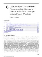
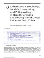
Acaseinpointistherelatively “thin”understandingbetweenroadconstruc-
tion and forest fragmentation that has developed for the Amazon Basin.
18
Figure 7.1
illustrates what is meant by a “thin” understanding and indicates where a “thick”
understandingneedstobedevelopedtomeettheneedsofconservationplanning.
Weacknowledgethatresearchinalimitednumberofcolonizationzonesinthe
Amazon Basin has modeled land colonization.
19,20,21,22
Thefociofthesestudieshas
generallybeenonsocietalprocessesandimpactsandontheresultingforestcoverin
a
general sense. Although this has deepened our understanding of land use dynamics
© 2008 by Taylor & Francis Group, LLC
Developing a Thick Understanding of Forest Fragmentation in Landscapes 121
in colonization zones, knowledge of the causal linkages between processes that lead
individual land owners to fragment the forests on their properties in particular ways,
and how the fragmentation patterns on individual properties mesh together across
acommunityoranumberofcommunities,hasrarelybeeninvestigated,though
itsimportanceisrecognized.
23,24
A notable exception is the research by Perz and
Walker
25

who applied a neo-Chayanovian analysis to secondary forest regrowth on
smallcolonistfarms,arguingthatmoreattentionneedstobepaidtohouseholdsas
themostproximatecontextinlandusedecisionmaking.
Forest
City A
City A
City B
City B
Conservation
unit
Major road
Flow of species between
conservation units
1
2
3
FIGURE 7.1 Thick and thin understandings of forest fragmentation along roads in lowland
forestsoftheAmazonBasin.Theprogressionfromstage1to2showsaforestblockdissected
byaroadconnectingcitiesAandB.Stage3illustrateslarge-scalefragmentationbetween
twoconservationunitsandtheconnectivitybetweenthemthatisrequiredisillustratedby
the black arrow. A “thin” understanding of fragmentation is represented in Stages 2 and 3;
the development of the “thick” understanding that we argue for in this chapter is required
forthewhiteareaalongthemainroad.
© 2008 by Taylor & Francis Group, LLC
122 Land Use Change
Ifplanningandmanagementinterventionsaretobemadeduringforestconver-
sioninareasundergoingcolonization,thenadetailedunderstandingofhowagentsare
operating in the landscape at different geographical scales is essential. For example,
the inuence of roads and other lines of access occur at one scale. Generalizations
abouttheenvironmentalimpactsofroadsatthisscalehavebeenrecognized

26,27,28
and used, somewhat contentiously, to model the impact of development policies in
Brazil.
29,30,31,32,33
Butnestedbelowtheroadnetworkingeographicalspaceisalmost
always a cadastre or land property grid. Although the roads can be constructed
both before and after a cadastre has been surveyed, we argue that the roads
and
the cadastre provide two spatial imprints connected through a scale hierarchy in
forested landscapes that are destined to fragment. Moreover, attempts to model frag
-
mentationspatiallybasedonroadbuildinghavemissedafundamentalpoint.That
is,itisthecolonisthouseholdswithinthelimitsoftheirpropertiesthatcreatethe
patternsofforestfragmentationbyrespondingtoeconomicandpolicysignalswith
machetesandchainsaws,ratherthanplannersandroadbuilderswithmapsand
bulldozers. It could be argued that the planners and road builders spatially constrain
what farmers can clear, as well as provide the wherewithal to extract timber and
produce from their farms. We acknowledge that the argument that we make here
mayonlyapplytofarmersinplannedcolonizationschemes:itmaynotapplytoother
types of humid tropical forest colonization in the Amazon Basin or elsewhere.
Developing a “thick” understanding of fragmentation at contemporary deforesta
-
tion fronts therefore requires integrating the actions of land managers on individual
properties over time and meshing them together within the road networks and land
property grids. In an applied vein, what is required specically to plan and manage
landscapes of colonization is research into the spatial and temporal dynamics of forest
fragmentation, which cover multiple scales, considering all agents of change, and the
links between agents and scales. The results of such research will allow an important
questiontobeanswered.Thatis,howdothecollectiveactionsoflandmanagersina
particular area lead to particular patterns of forest fragmentation over trajectories of

time? If this question can be answered robustly, then two further questions of concern
to landscape ecologists and conservation planners can also be tackled:
1. Canzonesofcolonizationbeplannedsothattheycandevelopintomulti-
purposelandscapesthatallowruralproductionsystemstoco-existwith
biological conservation?
2. How can existing, partially fragmented landscapes be planned for?
Inthischapterweexplainhowwehaveattemptedtodevelopa “thick”under
-
standing of the dynamics of landscape fragmentation in a colonization zone in the
lowlandhumidtropicsofBolivia,andthenreectonfurtherresearchneeds.
7. 2 CASE STUDY AND METHODS
7. 2.1
CHAPARE
We used observations from the Chapare region of Bolivia in this research. Chapare
is a colonization zone in the humid tropical lowlands of Bolivia dating back to the
© 2008 by Taylor & Francis Group, LLC
Developing a Thick Understanding of Forest Fragmentation in Landscapes 123
1930s, though most colonization and forest conversion has taken place since the
1960s.
34,35,36,37,38
Theareaisboundedtothenorthbyrelativelyundisturbedlowland
tropical forests and to the south by montane forests. These forests are likely to remain
relatively undisturbed in the foreseeable future because to the north they are either
permanently or seasonally inundated, and to the south they are protected by Parque
Nacional (PN) Carrasco. The zone of colonization creates a wedge of livelihoods and
disturbance between these two forest blocks, thereby compromising the exchange of
animalsand,lessobviously,plantmaterialbetweenthetwo.Giventhestrongafni
-
tiesbetweentheanimalsandplantsinthelowlandmontaneforestsinPNCarrasco
andthelowlandforests,thisisacauseofconcernforconservationists.

Chapare benets from a dense network of primary and secondary roads aug
-
mented by foot tracks.
34,37,39
This network has developed progressively since the 1960s
in two ways. First, by its physical extension; second, by upgrading the road surfaces
fromdirttotarmacorcobble.Alandpropertygridhasdevelopedinparallelwith
theroadnetwork,andthetwoareintegraltocolonizationofthearea.Thelandnow
occupiedbyeachofthecommunitiesinChaparewassurveyedandmarkedoutdown
tothelimitsofeachlandparcelbytheInstitutoNacionaldeColonización(INC)
beforeitwassettled.Titlesweregiventocolonistsmovingintoeachcommunity.
These records are held by INC. The transportation network and the land property
gridcombinetoprovidethespatialstageonwhichcolonistsactouttheirlivelihoods,
while simultaneously spatially constraining their activities.
7. 2.2 METHODS
Tounderstandthespatialandtemporalrelationshipsbetweenthedifferentagents
of change, one of us (Bradley) conducted detailed surveys in three communities
between 2000 and 2003.
34
SalientdetailsofeachcommunityarelistedinTable7.1.
Ineachcommunitythefollowingresearchwasundertakentodevelopanunder
-
standingofthespatialandtemporaldynamicsoflandcoverchange:
1. ThelandpropertygridforeachcommunitywasobtainedfromINCandthe
owners of each property identied.
2. Permissionwasobtainedfromthecommunity
sindicato to interview land
owners/managers. Subsequently those interviewed were selected randomly.
TABLE 7.1
Salient Information Concerning the Three Communities Studied

Community Area (ha)
Altitude
(m.a.s.l.)
Number of
properties
Year of first
settlement
Prevailing economic
activities 2000–2003
Arequipa 1,220 250 60 1983 Banana, black pepper,
cassava, heart of palm, and
rice cultivation
Bogotá 3,196 250–350 90 1972 Cattle rearing: beef and dairy
Caracas 1,745 220 110 1963 Banana, mandarin, and
orange cultivation
© 2008 by Taylor & Francis Group, LLC
124 Land Use Change
andETM+imageryacquiredinthedryseasonsof1975,1976,1986,1992,
1993,1996,and2000usingclassicationalgorithmsinERDASImagine
(fulldetailsofwhichcanbefoundinBradley
34
). Field verication was car-
These maps were then simplied into binary forest and nonforest covers.
nonforest maps for their property and asked to recall aspects of forest clear
-
anceandwhatcropshadbeengrownatthetimestheimageswereacquired.
This was done using participatory rural appraisal methods, the most infor
-
mative of which was to walk each farmer’s property with him. This enabled
farmers to verify their recall of what had been grown at particular times,

and also enabled geolocation of these observations using a global position
-
ingsystem(GPS)receiverinnondifferentialmode.
5. Foreachpropertysurveyed,aforest/nonforestmap—
a property forest/
nonforest map—wasannotatedwiththeowner/manager’sobservations.
Propertiesaretypically20hainareasofcultivationand50hainareasoflive
-
Bogotá, and Caracas, respectively (Table 7.1). The names of the communities and
the farmers we interviewed have been made anonymous in accordance with normal
social science survey practices, and because some of the farmers have illegally
grown coca in the past. The observations made about farms and farmer’s responses
to questions were used in two ways. First, to understand the drivers of land use
change in Chapare from the 1970s to the present time,
34
and second, to verify the
forest/nonforest maps of each community—
community forest/nonforest maps—that
the
property forest/nonforest maps of each property surveyed were extracted from.
The veried
community forest/nonforest maps were then used to map areas of forest
and nonforest for each community.
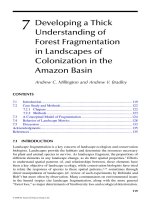
7. 3 A CONCEPTUAL MODEL OF FRAGMENTATION
By comparing the progressive development of spatial patterns of forest fragmenta-
tion between the three communities we developed a conceptual model of forest frag
-
mentation that has six phases (Figure 7.3). The rst or planning phase occurs before
colonization,and,consequently,noforesthasbeenclearedatthistime (Figure7.3a).
However,thisstageisimportantforitisatthistimethatthegeneralspatialcon

-
guration of forest and agriculture patches that will ultimately populate this
geographical space is determined. This is because the property grid is surveyed and
laid out, and the (unimproved) access roads and tracks are constructed. This phase
existsforashortperiodoftimebeforecolonistsarrive.Inthesecondphase—early
colonization—olonists clear forest at the primary ends of each property, thereby
creating a simple pattern of fragmentation on either side of the primary access road
(Figure 7.3b). In the three communities we researched intensively, all properties
wereoccupiedalmostimmediately,andtheareasofeachplotcleared(calculated
from
community forest/nonforest maps) were similar because the colonists either
arrived together or within a few months of each other. Moreover, their motivations
© 2008 by Taylor & Francis Group, LLC
3. LandcovermapsofeachcommunitywerecreatedusingLandsatMSS,TM,
stockrearing.Fifteen,13,and17propertiesweresurveyedindetailforArequipa,
4. Each land owner/manager selected was shown the time sequence of forest/
riedoutonthemapsderivedfromimageryacquiredin2000(Figure7.2).
Developing a Thick Understanding of Forest Fragmentation in Landsca
pes 125
TM Band 4 image: 11
th
April 1986 TM Band 4: 18
th
July 1993 ETM Band 4: 14
th
July 2000
FIGURE 7.2 Sequence of images showing progressive deforestation that is spatially constrained within a network of primary
and secondary feeder roads in between which are rectangular landholdings. The imagery is from eastern Chapare between 1986
and2000andis10by10kminarea;allimagesareatmosphericallyandgeometricallycorrectedTM/ETM+Band4.(a)Shows
the least forest clearance and was acquired on 11 April 1986. The dark gray tones that dominate the image are different types of

lowland tropical forest. The main Cochabamba-Santa Cruz bisects the image and forest is cleared about 500 m on either side of
theroad.Anetworkofprimaryfeederroadscanjustbeseenintheforestedareasoneithersideofthemainroad,althoughthere
is very little clearance in any of the communities these roads serve. The black sinuous pixels are small rivers that bisect Chapare
andemanatefromtheAndesfoothillstothesouthoftheimages.(b)Imagewasacquiredon18July1993.Thelightgrayareas
along the primary feeder roads are areas of clearance. (c) Image was acquired on 14 July 2000 and shows further deforestation.
Different size forest patches that have been isolated by deforestation fronts coalescing from different directions can be seen in
thecenteroftheimage.Thecastellatednatureofdeforestationinthistypeofcolonizationschemecanbeclearlyseen.
© 2008 by Taylor & Francis Group, LLC
126 Land Use Change
1819 20 21 22 2324 25 26 27 28 2930 31 32 33 34
1819 20 21 22 2324 25 26 27 28 2930 31 32 33 34
1 2 4 5 6 7 8 910111213141516173
1 2 4 5 6 7 8 910111213141516173
18 19 20 21 22 2324 25 26 27 28 2930 31 32 33 34
B
A
C
C
1 2 4 5 6 7 8 910111213141516173
18 19 20 21 22 2324 25 26 27 28 2930 31 32 33 34
B
A
C
1 2 4 5 6 7 8 910111213141516173
1819 20 21 22 2324 25 26 27 28 2930 31 32 33 34
18 19 20 21 22 2324 25 26 27 28 2930 31 32 33 34
C
B
A
1 2 4 5 6 7 8 9 10111213141516173 1 2 4 5 6 7 8 9 10111213141516173

Stream
Property
grid
Primary
access
road
Secondary
access
road(s)
(a)
(b) (e)
(f)(c)
(d)
FIGURE 7.3 Six-phase conceptual model of forest fragmentation based on a community
with 34 plots (numbered 1 to 34) of equal area. A primary access road (black) runs through
thecenterofthecommunityandastreamcutsthroughproperties1to7.Imagesrepresent:
(a) the planning phase, (b) the early colonization phase, (c) the illicit coca phase, (d) the
improved access phase with secondary roads (gray roads), (e) the complex clearance phase,
and (f) the plot exhaustion phase. The light gray cells in phases (e) and (f) represent secondary
regrowth forest.
© 2008 by Taylor & Francis Group, LLC
Developing a Thick Understanding of Forest Fragmentation in Landscapes 127
forclearanceweresimilar,thatis,toclearforestforlandtoplantsubsistencecrops
(followed by cash crops in subsequent years) and to acquire construction materials
forhouses.Inaless-detailedexaminationoftheimageseriesforallofChapare,we
sawthisphasereplicatedinallcommunities.
More complex spatial patterns of forest fragmentation establish themselves in
the third phase of the model—the illicit coca cultivation phase (Figure 7.3c). Because
coca cultivation in the lowlands of Bolivia has always been illegal (in comparison to
cultivationforchewinginthesubtropicalmontaneforestswhereitislegal),farmers

generally adopted strategies to cultivate coca that fragmented forests in particular
ways. However, in the 1970s when coca cultivation and cocaine production was
barely controlled by the government, coca was grown openly at the primary ends
of many properties. As government crackdowns on coca growing took effect, many
farmers grew
legal cash and subsistence crops at the primary ends of their plots and
retreated into the remaining forest on their properties to clear small areas to grow
coca. This was the main cause of forest perforation, and the extent of perforation
depicted in this model (Figure 7.3c) is high because of illegal coca cultivation and
is probably greater than it would be in other colonization areas. This assumption
has yet to be tested. The colonist footprint model developed by Brondizio et al.
20
predictshighratesofforestclearanceatthisstageasfarmerspreparelandtoplant
perennial cash crops. But our evidence indicates that although a few farmers cleared
forestatmuchfasterratesthanothers(e.g.,property28,Figure7.3c),thiswasexcep
-
tionalbecausethevastmajorityoffarmersonlyhadtoclearsmallareastocultivate
theperennialcropofchoice—coca—which,becauseithasahigh-sellingreturn,is
conservativeinitslandrequirements.Differencesinforestclearanceratesbetween
individual properties occur at this stage because few farmers cultivated land-hungry
perennialcropsatthistime,aspredictedbyBrondizioetal.,
20
rather than coca.
These differences lead to the castellated pattern of the forest/nonforest boundaries
that characterize “shbone” deforestation.
Thedevelopmentofsecondary,unimprovedfeederroadsatsomepointintime
duringcolonizationistypicalofmostcommunitiesinChapare.Roadsandtracksare
constructed along the boundaries of communities to connect with the roads that were
constructedinitially.Wehavecharacterizedthisphaseasimprovedaccess,andin
1to11and18to27.Theestablishmentofsuchroadsandtracksallowsplotstobe

cultivatedfrombothends,buttheactualreasonsfortheirconstructionareunclearat
present. Our interviews so far suggest they may be constructed to consolidate com
-
munity boundaries, but they may simply improve access. Whatever the reason, they
can be used to split up properties to satisfy actual and potential disputes over inheri
-
tance, or allow farmers to cultivate more fertile soils at one end of their property
whileallowingrecoveryofvegetationandsoilattheotherendoftheplot.
Inthefthphaseofthemodel—complexclearance—asignicantamountofthe
landinacommunityisundersometypeofcultivation(Figure7.3e).Thetermcomplex
arises because many landscape ecology metrics attain their highest values during this
phase. The formation of both forest patches and the extension of the forest perimeter
are due to differential rates of clearance between farmers, and the continuation of
forest clearance from both the primary and secondary ends of some properties. The
© 2008 by Taylor & Francis Group, LLC
Figure 7.2d secondary feeder roads are drawn along the secondary end of properties
128 Land Use Change
formationofaforestpatchduetothedifferencesinratesofforestclearanceisshown
inFigures7.3dand7.3e.Thefarmersinproperties21and23haveclearedforestat
fasterratesthanthefarmerinproperty22.Asaconsequenceapatchofforest(B)on
property22,whichonceshieldedacocaclearing(A),isnowsurroundedbyagricul
-
tural land. This method of patch formation is commonplace in Chapare, and occurs
because of the intersection of government coca eradication policies (which causes
perforation-style clearance of forest deep in properties), differences in crop choices
betweenfarmers(whichleadstodifferentlandrequirementstogrowparticularcrops),
and differences in household circumstances and aspirations. The creation of forest
patchConproperty10isavariantonthewayinwhichforestpatchBwasformed.In
this case the rates of forest clearance between properties 9, 10, and 11 are not only dif
-

ferentintheamountsofforestclearedannually,butalsothedirectionsofclearanceare
different because of the inuence of the secondary access road on property 9.
We have termed the nal phase plot exhaustion (Figure 7.3f). By this we mean that
most of the forest has been cleared. Some isolated patches remain, and there are also
patches of secondary regrowth forest and forests in areas that are difcult to clear or are
located on land that cannot be cultivated (e.g., the riparian forest in properties 1 to 7).
We have evidence that properties are already changing hands by the time
thepenultimateandnalstagesofthemodelarereached.Althoughwehavenot
recorded land being sold in the 45 properties we have surveyed in detail, we have
come across this on farms we have visited in other communities. Some properties
arebeingsoldtonewownersandsomewealthyfarmerspurchaseadjacentplots
toincreasetheircontiguouslandholdings.Wehaveindicatedthisinthemodelby
combining properties 28 and 29 in Figure 7.3f.
7.4 BEHAVIOR OF LANDSCAPE METRICS
Theconceptualmodeloutlinedaboveisbasedondetailedobservationsmadein
threecommunities,andtoevaluateitsutilityforanalyzingtheecologicalimplica
-
tions of fragmentation we used metrics commonly employed by landscape ecologists
and conservation biologists. We calculated proportional forest cover, the number
of forest patches, and the forest/nonforest edge length for each phase in the model
Lambin
11
postulated that landscape metrics used to characterize fragmentation
would follow a particular trajectory as tropical forest landscapes changed from those
that were entirely forested, through landscapes of agricultural patches in a forest
matrix,toentirelyagriculturallandscapes(i.e.,afewforestpatchesinanagricul
-
turalmatrix).Hedidnotquantifythispostulatedbehavior,buthypothesizedthat
themetricswouldattainpeakvaluesintheheterogeneous,intermediatelandscapes
and would be low for homogenous forest or agricultural landscapes. Trani and

Giles
40
simulated deforestation of a hypothetical forest and calculated metrics at
variouspointsalongadeforestation/fragmentationtrajectory.Threemetricsfrom
their analysis—mean forest patch size, the forest/nonforest edge length, and the
mean nearest neighbor distance between forest patches—are shown in Figure 7.5.
We calculated the same landscape ecology metrics as Trani and Giles
40
for each
communitywestudiedusingFragstats.
41
As the metrics followed similar trends in
each community, we only illustrate the metrics for Communidad Arequipa in this
© 2008 by Taylor & Francis Group, LLC
(Table7.2).ThesedataarevisualizedinFigure7.4.
Developing a Thick Understanding of Forest Fragmentation in Landscapes 129
TABLE 7.2
Selected Landscape Metrics Calculated for the Six Phases of the
Conceptual Model
Phase in
conceptual model
Proportional
forest loss
(%)
Number of
forest
patches
Number of
cultivation
patches

Mean patch
size (nominal
units)
Forest edge
length
(nominal units)
Planning 0 1 0 306 0
Early colonization 10.8 2 1 137 37
Illicit coca 29.7 4 20 71 140
Improved access 36.6 6 15 49 151
Complex clearance 58.8 12 7 11 203
Plot exhaustion 83.3 20 2 3 135
100
350
300
250
200
150
100
50
80604020
Mean patch size
100
250
200
150
100
50
80604020
Total forest edge length

Proportion of forest cleared (%)
(b)
Proportion of forest cleared (%)
(a)
FIGURE 7.4 Metricscalculatedfortheconceptualmodel:(a)meanforestpatchsize,and
(b)totaledgelength.Bothareinnominalunits.
© 2008 by Taylor & Francis Group, LLC
130 Land Use Change
10080604020
Mean patch size (km
2
)
1000
800
600
400
200
Total forest edge length (km)
MNN distance between
forest patches (km)
10080604020
250
200
150
100
50
10080604020
1.2
1.0
0.8

0.6
0.4
0.2
Proportion of forest cleared (%)
(a)
Proportion of forest cleared (%)
(b)
Proportion of forest cleared (%)
(c)
FIGURE 7.5 Selected metrics from Trani and Giles
40
:(a)meanforestpatchsizeinkm
2
,
(b)totaledgelengthinkm,and(c)meannearestneighbordistancebetweenforestpatches
in km.
© 2008 by Taylor & Francis Group, LLC
Developing a Thick Understanding of Forest Fragmentation in Landscapes 131
chapter(Figure7.6)and,asforestlosshadonlyreached46%by2000forthiscom-
munity,thedatadonotextendtoveryhighproportionalforestlosses.Comparing
the limited number of metrics in Figures 7.4, 7.5, and 7.6 provides an initial test
oftherobustnessoftheconceptualmodel.Adeclineinforestcoverovertimein
the conceptual model is clear in Table 7.2. This allows the successive phases of the
model to be parameterized as proportional forest losses in the graphs in Figure 7.4.
Both Lambin
11
and Trani and Giles
40
usedforestcoverintheirgraphs.
Mean patch size declines in a consistent manner (Figures 7.4a, 7.5a, and 7.6a).

Initially the decline is rapid, more so in reality (in Communidad Arequipa) than in
the model or the simulation. At around half the area deforested, the rate of decrease in
meanpatchsizedeclinesandthentherateofdecreaseinforestpatchsizetapersoff.
Totaledgelengthinitiallyincreasesasforestsbegintobecleared,andtheedgelength
is at its greatest at intermediate forest covers and then declines. This is evident in the
conceptual model, the simulation, and in the real data, Figures 7.4b, 7.5b, and 7.6b,
respectively.Therearedifferencesinthepeakvaluesoftotaledgelength,whichsuggest
the variation in the peak may be related to the spatial conguration of fragmentation.
Whereas Trani and Giles
40
simulated a somewhat random pattern of fragmentation,
that in Communidad Arequipa and the simulation model are for regularly structured
landscapes,which,becausepropertiesarelongandthin,hasatendencytohavehigh
edge lengths at intermediate forest losses compared to lower edge lengths in more
randomly fragmented forests. The third metric—mean nearest neighbor (MNN) dis
-
tance between forest patches—has only been calculated for the actual data from Com
-
munidadArequipa andextractedfromTraniandGiles’s
40
simulation. For this metric
thereisadifferenceinbehavior.ThereisrelativelylittlevariationintheMNNdis
-
tanceinCommunidad Arequipa,andthedistancesovertherangeofforestcoversin
the community describe a shallow U-shape. However, Trani and Giles’s simulation
describes an upturned-U distribution in MNN distance as forest is progressively lost.
In summary, our analysis of landscape metrics suggests that:
1. Mean patch size (MPS) and total edge length (TEL) are very robust and
consistent measures of fragmentation. Although in all three cases there are
similar trends in MPS and TEL with progressive deforestation and increas

-
ingforestfragmentation,therearedifferencesintheprecisenatureofthe
curves, which may be a function of the effect that the spatial conguration
of land properties have on fragmentation. From the viewpoint of model
validation the latter point is not that important, but it does lend weight to
theargumentthatunderstandinglandowner’sdecisionsatthesmallscale
is important for developing our understanding of fragmentation and future
planning of colonization zones.
2. The behavior of the mean nearest neighbor distance between forest patches
does,however,varybetweenthestudiesandisdueeithertothediffer
-
encesinspatialscalebetweenthetwostudiesorthenatureofforestloss.
In Communidad Arequipa the spatial imprint of the cadastral grid and the
waysinwhichpeopleclearforestwithinthegridmayleadtoarestricted
set of possible distances between forest patches and, as these have only
been observed in the early stages of fragmentation, they may change sig
-
nicantlyasmoreforestisclearedandfragmentationproceeds.
© 2008 by Taylor & Francis Group, LLC
132 Land Use Change
10080604020
Mean patch size (km
2
)
MNN patches (km
2
)
60
50
40

30
20
10
Total forest edge length (km)
10080604020
120
100
80
60
40
20
10080604020
60
50
40
30
20
10
Proportion of forest cleared (%)
(a)
Proportion of forest cleared (%)
(b)
Proportion of forest cleared (%)
(c)
FIGURE 7.6 Metrics calculated for Communidad Arequipa: (a) mean forest patch
size in km
2
,(b)totaledgelengthinkm,and(c)meannearestneighbordistance
between forest patches in km.
© 2008 by Taylor & Francis Group, LLC

(a) (b)
(c) (d)
PCA classes
1
2
3
4
5
6
7
8
9
10
11
12
13
14
15
16
17
18
19
20
21
22
St. Dev. NEP
0.004
–
0.027
0.027

–
0.05
0.05
–
0.073
0.073
–
0.096
0.096
–
0.118
0.118
–
0.141
0.141
–
0.164
0.164
–
0.187
0.187
–
0.21
0.21
–
0.233
NEP 8593
<
–
2

–
2
––
1
–
1
––
0.5
–
0.5
––
0.2
–
0.2
–
0
0
–
0.2
0.2
–
0.5
0.5
–
1
>
1
NEP 9400
<
–

2
–
2
––
1
–
1
––
0.5
–
0.5
––
0.2
–
0.2
–
0
0
–
0.2
0.2
–
0.5
0.5
–
1
>
1
FIGURE 2.4 (a) The spatial pattern of temporal signals may be grouped by applying prin-
cipal components analysis to the time series and creating a classication based on the major

principal components. (b) The temporal metrics may be calculated on the spatial times series
to create maps of, for example, standard deviation of net ecosystem productivity (NEP). (c) A
running integration, trend, or wavelet analysis may dene periods of distinct behavior in the
time series that can then be summarized by metrics such as an integral of NEP for periods of
decline and increase. Shown for 1985–1993 and 1994–2000 here.
© 2008 by Taylor & Francis Group, LLC
(a) (b)
(c) (d)
Cattle distribution
VRD
Vegetation polygons
Grassland classes
Other forest and bush
Sorghum woodland
–
low SUR
Sehima woodland
–
moderate SUR
Triodia woodland
–
low utilisation potential
Dicanthium grassland
–
high SUR
Triodia grassland
–
low utilisation potential
Mitchell grassland
–

very high SUR
Aristida woodland
–
Imoderate SUR
Not rangeland
VRD
No. threatened birds
0
1
2
3
4
VRD
Mines
0
1
2
5
VRD
PFE ($)
NA
–
1
0
1
2
3
4
Cattle
Not grazed

Water points
Victoria River
District
Roads/Rivers
FIGURE 2.5 Temporal signals are usually based on biophysical or human phenomena that
operate at a large scale (e.g., climate, interest rates). Demographic changes at a ne scale may
have scale limitations due to level of aggregation in reporting. Temporal signals and indica-
tors are ltered by spatial variation. The Victoria River District in the Northern Territory
of Australia is highly productive. (a) Cattle are distributed of freehold-leasehold land but
conned by water points. (b) Both productivity and ecological impact vary with vegetation
type, which is associated with soils, topography, and rainfall gradient. (c) Costs are low and
enterprises are protable but the increment is small on a per hectare basis. (d) Mining with
major physical disturbance occurs sporadically across the area. There are threatened bird
species in the region and these may be ground nesting and impacted by grazing.
© 2008 by Taylor & Francis Group, LLC
Potential productivity for grazing
Rainfall reliability
Rainfall rel. (w/sp)
Rainfall rel. (ann)
Forage potential
Growth Foliage proj cover Soil nutrient
Accessibility (ARIA)
Soil PSoil NSoil carbon
NDVI meanNPP mean
soil_fert
FIGURE 2.7 Cognitive mapping interface suitable for combination of diverse spatiotemporal metrics, indices,
and data layers describing meaningful properties of a system under analysis. This example shows the construction
of a composite index to represent potential grazing productivity from rangelands.
46,58
© 2008 by Taylor & Francis Group, LLC

© 2008 by Taylor & Francis Group, LLC
FIGURE 3.1 Land use change in the Barmera, Berri, and Renmark areas of South Australia.
Statistical Local Areas
Irrigated horticulture first mapped prior to 1990 (mapped in 1988 for SA)
Irrigated horticulture first mapped in 1995 and between 1990
–
1995
Irrigated horticulture first mapped between 1995
–
1999
Irrigated horticulture first mapped in 2001
Irrigated horticulture first mapped in 2003
Irrigated horticulture data provided by
SA Department of Environment and Heritage
Loxton
Berri
Barmera
Renmark
© 2008 by Taylor & Francis Group, LLC
N
S
WE
Kilometers
Land managers who did not identify salinity
0
–
0.045625827
0.045625827
–
0.091251653

0.091251653
–
0.136877480
0.136877480
–
0.182503307
0.182503307
–
0.228129134
0.228129134
–
0.273754960
0.273754960
–
0.319380787
0.319380787
–
0.365006614
0.365006614
–
0.410632440
0.410632440
–
0.456258267
Glenelg Hopkins region
No (land manager identified salinity)
Yes (land manager identified salinity)
Salinity discharge sites
Land managers who identified salinity
Std. Dev = 6674.11

Mean = 6369
N = 702.00
Std. Dev = 4146.41
Mean = 2536
N = 290.00
36,000
–
38,000

32,000
–
34,000
28,000
–
30,000
24,000
–
26,000
20,000
–
22,000

16,000
–
18,000
12,000
–
14,000
8,000
–

10,000
4,000
–
6,000
0
–
2,000
36,000
–
38,000
32,000
–
34,000

28,000
–
30,000
24,000
–
26,000
20,000
–
22,000
16,000
–
18,000
12,000
–
14,000
8,000

–
10,000
4,000
–
6,000
0
–
2,000
Distance to nearest salinity discharge site (meters)
Distance to nearest salinity discharge site (meters)
Frequency
0 30 60 120
300
200
100
0
Frequency
300
200
100
0
Distance to nearest salinity discharge site
<
VALUE
>
Legend
FIGURE 3.3 Land managers’ perception of salinity and mapped salinity discharge sites.
© 2008 by Taylor & Francis Group, LLC
N
S

WE
Kilometers
0
–
0.012443533
0.012443533
–
0.024887066
0.024887066
–
0.037330598
0.037330598
–
0.049774131
0.049774131
–
0.062217664
0.062217664
–
0.074661197
0.074661197
–
0.087104730
0.087104730
–
0.099548262
0.099548262
–
0.111991795
0.111991795

–
0.124435328
Glenelg Hopkins region
Farmer
Non
–
farmer
Conservation of natural environments
Std. Dev = 1595.02
Mean = 1951
N = 640.00
Std. Dev = 1249.48
Mean = 1276
N = 355.00
8000
–
8500
7000
–
7500

6000
–
6500

5000
–
5500
4000
–

4500
3000
–
3500
2000
–
2500
1000
–
1500
0
–
500
8000
–
8500
7000
–
7500
6000
–
6500
5000
–
5500
4000
–
4500
3000
–

350
0
2000
–
2500
1000
–
1500
0
–
500
Distance to nearest area of high conservation value (meters)
Distance to nearest area of high conservation value (meters)
Non
–
farmer
Farmer
Frequency
0 30 60 120
Frequency
140
120
100
80
60
40
20
0
140
120

100
80
60
40
20
0
Distance to nearest area of high conser vation value
<
VAL UE
>
Legend
FIGURE 3.4 Land managers who manage properties near areas of high conservation value.
© 2008 by Taylor & Francis Group, LLC
FIGURE 5.3 Predicted
deforestation hot spots
obtained by combining
areas predicted to have
the highest probability of
forest conversion (>70%)
from the best model (the
region-specic classica-
tion tree) with the areas
with greater than 2% rural
population growth rate
(1985–1993). Red depicts
the deforestation hot spots
(areas with >70% proba-
bility of forest conversion
and >2% rural population
growth). Orange and red

depict areas with >70%
probability of forest con-
version. Green depicts
forested areas, gray rep-
resents cleared forested
areas, and white repre-
sents nonforested areas.
White circled areas indi-
cate current hot spots of
deforestation, which are also areas of high-value biodiversity value: (1) Quibdó-Tribugá,
(2) Farallones-Micay, (3) Patía-Mira, (4) Fragua-Patascoy, (5) Alto Duda-Guayabero,
(6) Macarena, (7) Guaviare, and (8) Perijá. Black line is the Andean region, and light
green lines are national parks. (From Etter et al.
50
With permission.)
N
S
WE
Kilometers
Major road
All
–
year road
Water body
Ye s
No
05025 100 150
Legend
Tanzania
Rwanda

Kenya
Sudan
Congo, DRC
Kampala
North
Central
East
West
Deforestation
FIGURE 4.1 Uganda study area showing the distribution of
deforestation within the western region of the country.
N
Km5002500
1
2
3
4
5
6
7
8
© 2008 by Taylor & Francis Group, LLC
Forest cover zone (%)
Cleared
1989
(a)
(b)
1996 1999 2002
Forest
0

–
10 10
–
20 20
–
30 30
–
40 40
–
50 50
–
60 60
–
70 70
–
80 80
–
90 90
–
100
FIGURE 5.4 Forest maps of the colonization front for each study date: (a) extent of forest cover (black = forest); and (b) percentage
forest cover at 10% increment zones. (From Etter et al.
39
With permission.)
© 2008 by Taylor & Francis Group, LLC
LEGEND
Rapid deforestation
Rapid forest regeneration
Minor changes
To w ns

Rivers
Roads
1999
–
2002 military
exclusion zone
1989
–
1996 1996
–
1999 1999
–
2002
FIGURE 5.5 Spatial location of the local hot spots of deforestation (red) and regeneration (green) for the three time periods of
study. (From Etter et al.
39
With permission.)
© 2008 by Taylor & Francis Group, LLC
IJI = 14.2
MPS = 8.1
IJI = 17.9
MPS = 4.7
IJI = 23.7
MPS = 2.2
IJI = 19.2
MPS = 3.1
(2)
(2a)
(2b)
(3a)

(3)
(1)
FIGURE 6.1 The panel process, conducted at both the pixel and patch levels: (1) four multi-
spectral satellite images are each categorized into a thematic LULC classication; (2) pattern
metrics are run on each of the four LULC classications, each producing a set of patch, class,
and landscape statistics (here the interspersion/juxtaposition index [IJI] and mean patch
size [MPS] are shown) as well as an output image of the delineated patches; (2a) pattern
metric output for each of the four times is used to calculate three piecemeal change maps for
each pattern metric and each consecutive pair of images (e.g., showing uctuations in IJI or
MPS between two time periods) as per Crews-Meyer
11,27
; (2b) three pattern change maps are
stacked into one panel of all structural change for each given metric (e.g., showing uctuation
in IJI or MPS through all time periods) as per Crews-Meyer
11,27
; (3) three thematic change
maps are created for each of the time periods represented by the four classications; (3a) the
three thematic change maps are stacked to represent the full record of all thematic change
across the four classications as per Crews-Meyer.
3
© 2008 by Taylor & Francis Group, LLC
FIGURE 6.3 (a) LULC in the greater study area in the 1972/1973 water year; (b) 1985; and (c) 1997.
© 2008 by Taylor & Francis Group, LLC