WETLAND AND WATER RESOURCE MODELING AND ASSESSMENT: A Watershed Perspective - Chapter 10 potx

Part III
Water Quality and
Biogeochemical Processes
© 2008 by Taylor & Francis Group, LLC
115
10
Estimating Nonpoint
Source Pollution
Loadings in the Great
Lakes Watersheds
Chansheng He and Thomas E. Croley II
10.1 INTRODUCTION
Nonpoint source pollution is the leading source of impairment of U.S. waters (U.S.
Environmental Protection Agency [EPA] 2002). In the Great Lakes basin, contam-
inated sediments, urban runoff and combined sewer overows (CSOs), and agri-
culture have been identied as the primary sources of impairments of the Great
Lakes shoreline waters (U.S. EPA 2002). The problems caused by these pollutants
include toxic and pathogen contamination of sheries and wildlife, sh consumption
advisories, drinking water closures, and recreational restrictions (U.S. EPA 2002).
Management of these problems and rehabilitation of the impaired waters to shable
and swimmable states require identifying impaired waters that are unable to sup-
port sheries and recreational activities and tracking sources of both point and non-
point source material transport through a watershed by hydrological processes. Such
sources include sediments, animal and human wastes, agricultural chemicals, nutri-
ents, and industrial discharges, and so forth. While a number of simulation models
have been developed to aid in the understanding and management of surface runoff,
sediment, nutrient leaching, and pollutant transport processes such as ANSWERS
(Areal Nonpoint Source Watershed Environment Simulation) (Beasley and Huggins
1980), CREAMS (Chemicals, Runoff and Erosion from Agricultural Management
Systems) (Knisel 1980), GLEAMS (Groundwater Loading Effects of Agricultural
Management Systems) (Leonard et al. 1987), AGNPS (Agricultural Nonpoint

Source Pollution Model) (Young et al. 1989), EPIC (Erosion Productivity Impact
Calculator) (Sharpley and Williams 1990), and SWAT (Soil and Water Assessment
Tool) (Arnold et al. 1998), to name a few, these models are either empirically based,
or spatially lumped, or do not consider nonpoint sources from animal manure and
combined sewer overows (CSOs) and infectious diseases. To meet this need, the
National Oceanic and Atmospheric Administration (NOAA) Great Lakes Environ-
mental Research Laboratory (GLERL) and Western Michigan University are jointly
developing a spatially distributed, physically based watershed-scale water quality
model to estimate movement of materials through both point and nonpoint sources in
both surface and subsurface waters to the Great Lakes watersheds. The water quality
© 2008 by Taylor & Francis Group, LLC
116 Wetland and Water Resource Modeling and Assessment
model evolves from GLERL’s distributed large basin runoff model (DLBRM) (Croley
and He 2005; Croley et al. 2005). It consists of moisture storages of upper soil zone,
lower soil zone, groundwater zone, and surface, which are arranged as a serial and
parallel cascade of “tanks” to coincide with the perceived basin storage structure.
Water enters the snowpack, which supplies the basin surface (degree-day snowmelt).
Inltration is proportional to this supply and to saturation of the upper soil zone
(partial-area inltration). Excess supply is surface runoff. Flows from all tanks are
proportional to their amounts (linear-reservoir ows). Mass conservation applies for
the snow pack and tanks; energy conservation applies to evapotranspiration. The
model allows surface and subsurface ows to interact both with each other and with
adjacent-cell surface and subsurface storages. Currently, it is being modied to add
materials runoff through each of the storage tanks routing from upper stream down-
stream to the watershed outlet (for details of the model, see the companion paper
by Croley and He 2006). This paper describes procedures for estimating potential
loadings of sediments, animal manure, and agricultural chemicals into surface water
from multiple databases. These estimates will be used as input to the water quality
model to quantify the combined loadings of agricultural sediment, animal manure,
and fertilizers and pesticides to Great Lakes waters for identifying the critical risk

areas for implementation of water management programs.
10.2 STUDY AREA
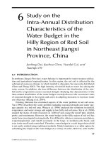
The study area of this research is the Cass River watershed, a subwatershed of the
Saginaw Bay watersheds. The Cass River watershed runs cross Huron, Sanilac, Tus-
cola, Lapeer, Genesee, and Saginaw counties of Michigan and joins the Saginaw
River near Saginaw (Figure 10.1) and has a drainage area of 2,177 km
2
. The Cass
River is used for industrial water supply, agricultural production, warm-water sh-
ing, and navigation. Agriculture and forests are the two major land uses/covers in the
Cass River watershed, accounting for 60% and 21% of the total land area, respec-
tively. Soils in the watershed consist mainly of loamy and silty clays and sands, and
are poorly drained in much of the area. Major crops in the watershed include corn,
soybeans, dry beans, and sugar beets. Over the years, the primary agricultural land
use and associated runoff, improper manure management, poor municipal wastewa-
ter treatment, irrigation withdrawal, and channel dredging and straightening have
led to high nutrient runoff, eutrophication, toxic contamination of sh, restrictions
on sh consumption, loss of sh and wildlife habitat, and beach closures in the Cass
River watershed (Michigan Department of Natural Resources 1988). Because of
dominant agricultural land use and related high soil loss potential, the Cass River
watershed was selected as the study area for estimating the loading potential of agri-
cultural nonpoint sources to assist the management agencies in planning and manag-
ing NPS (nonpoint source) pollution control activities on a regional scale.
10.3 ESTIMATING SOIL EROSION POTENTIAL
Soil erosion is caused by raindrops, runoff, or wind detaching and carrying soil par-
ticles away. It is the most signicant nonpoint source pollution factor affecting the
© 2008 by Taylor & Francis Group, LLC
Estimating Nonpoint Source Pollution Loadings 117
quality of water resources in the United States. Soil erosion by water includes sheet
and rill erosion. Sheet erosion is removal of a thin layer of soil from the surface of

the land. Rill erosion is removal of soil from the sides and bottoms of small channels
formed where surface runoff becomes concentrated and forms tiny streams. Sheet
erosion and rill erosion usually occur together and are hence referred to as sheet-
and-rill erosion (Beasley et al. 1984). Soil erosion by wind is the removal of soil by
strong winds blowing across an unprotected soil surface. This study focuses on the
potential of sheet-and-rill erosion by both water and wind at the watershed scale.
10.3.1 WATER EROSION POTENTIAL
The universal soil loss equation (USLE) (equation 10.1) is one of the most fundamental
and widely used methods for estimating soil erosion and sediment loading on an annual
basis (Wischmeier and Smith 1978). A number of simulation models, such as ANSWERS,
EPIC, AGNPS, and SWAT, use the USLE for erosion and sediment simulation.
Y = R*K*LS*C*P*Slope Shape (10.1)
OSCEOLA
ROSCOMMON
OGEMAW
IOSCO
ARENAC
GLADWINCLARE
MECOSTA ISABELLA
MIDLAND
BAY
HURON
TUSCOLA
SANILAC
LAPEER
GENESEE
SAGINAW
GRATIOTMONTCALM
SHIAWASSEE
OAKLAND

LIVINGSTON
Saginaw River
Legend
Kilometers
County Boundary
Watershed Boundary
Stream
50 0 50 100
Shiaivassee Rive
r
Flint River
Tittawassee Rive
r
Cass River
Saginaw
B
ay
N
FIGURE 10.1 The Saginaw Bay watershed boundary.
© 2008 by Taylor & Francis Group, LLC
118 Wetland and Water Resource Modeling and Assessment
where Y is the computed average soil loss per unit area, expressed in tons/acre; R is
the rainfall and runoff factor and is the rainfall erosion index (EI) plus a factor for
runoff from snowmelt or applied water; K is the inherent erodibility of a particular
soil; L is the slope length factor, S is the slope steepness factor; C is the cover and
management factor; P is the support practice factor; and the slope shape factor rep-
resents the effect of slope shape on soil erosion (Wischmeier and Smith 1978, Young
et al. 1989).
Realizing that the USLE is not intended for estimating erosion and sediment
yield from a single storm event, we use AGNPS to estimate the soil erosion and sedi-

ment potential for illustration purposes since we have not incorporated the revised
USLE (RUSLE) (Foster et al. 2000) into the distributed water quality model yet (He
et al. 1993, 1994). AGNPS, based on the USLE, simulates runoff, erosion and sedi-
ment, and nutrient yields in surface runoff from a single storm event. Basic databases
required for the AGNPS model include land use/land cover, topography, water fea-
tures (lakes, rivers, and drains), soils, and watershed boundary (He et al. 1993; 1994;
2001; He 2003). The model output includes estimates of runoff volume (inches),
sediment yield (tons), sediment generated within each cell (tons), mass of sediment
attached and soluble nitrogen in runoff (lbs/acre), and mass of sediment attached and
soluble phosphorus in runoff (lbs/acre).
The Digital Elevation Model (DEM) of 1:250,000 from the U.S. Geological Sur-
vey was used to derive slope and aspect. The STATSGO (State Soil Geographic Data
Base) data from the U.S. Department of Agriculture Natural Resources Conservation
Service were used to determine dominant texture, hydrologic group, and weighted
soil erodibility. The 1979 land use/land cover data from the Michigan Resource
Information System (MIRIS) and related hydrography databases were used to derive
land use–related parameter values. The storm event chosen was a 24-hour precipita-
tion of 3.7 inches with an average recurrence of 25 years. Fallow, straight-row crops,
and moldboard plow tillage were assumed in the simulation.
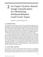
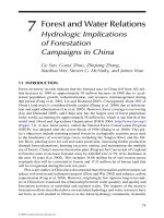
The model was applied to the Cass River watershed with a spatial resolution
of 125 ha (310 acres). (Note: the cell size was set at 310 acres to ensure the entire
watershed was discretized to no more than 1,900 cells—the limit of AGNPS ver-
sion 3.65.) The simulated results show that the runoff volume was higher in the
agricultural land (Figure 10.2). The soil erosion rate simulated from the single storm
event generally centered around 1 to 1.5 tons per acre, with no or little erosion in the
forested areas and a greater rate (up to 5 tons per acre) in portions of the agricultural
land. The sediment yield was highest (up to 45,000 tons in the 310-acre area) near the
mouth of the watershed as the atness of the area and lower peak runoff rate resulted
in a higher rate of deposition. These results indicate that agricultural activity was a
main nonpoint source pollution contributor under the worst management scenario

(fallow, straight-row crops, and moldboard plow tillage) (He et al. 1993).
10.3.2 WIND EROSION POTENTIAL
Wind erosion results in more than ve million metric tons of soil erosion, accounting
for 63% of the total soil erosion in the Saginaw Bay watersheds (Michigan Depart-
ment of Natural Resources 1988). The critical months for wind erosion are April and
© 2008 by Taylor & Francis Group, LLC
Estimating Nonpoint Source Pollution Loadings 119
May in the Saginaw Bay basin. Few methods are available for estimating soil ero-
sion by wind, such as the wind erosion equation developed by the U.S. Department
of Agriculture (USDA), Agricultural Research Service Wind Erosion Laboratory
(Woodruff and Siddoway 1965, Gregory 1984, Presson 1986). These methods are
suitable for estimating wind erosion potential at the eld level but difcult to use at
the watershed level. As soil erodibility, wind, and quantity of vegetative cover are the
main factors affecting wind erosion (Woodruff and Siddoway 1965), this study used
soil association data and vegetation indices to estimate the wind erosion potential for
the entire Cass River watershed.
STATSGO was used to extract six wind erodibility indices for all the soil asso-
ciations in the Cass River watershed. These groups are (USDA Soil Conservation
Service 1994):
Group 1: 310 ton/acre/year
Group 2: 134 ton/acre/year
Group 3: 86 ton/acre/year
Group 4: 56 ton/acre/year
Group 5: 48 ton/acre/year
Group 6: 38 ton/acre/year
These indices represent the wind erodibility based on the soil surface texture and
percentage of aggregates.
N
Soil Erosion (tons/acre)
0–0.2

0.2–0.5
0.5–0.95
0.95–1.81
1.81–4.76
FIGURE 10.2 Simulated soil erosion rate (tons/acre) from a 24-hour, 3.7-inch single storm
event in the Cass River watershed. (See color insert after p. 162.)
© 2008 by Taylor & Francis Group, LLC
120 Wetland and Water Resource Modeling and Assessment
The LANDSAT 5 TM data of June 1, 1992 was used to derive the Normalized
Differential Vegetation Indices (NDVI). These indices give a relative quantication
of vegetation amount, with vegetated areas yielding high values, and nonvegetated
areas yielding low or zero values. The formula for calculating the NDVI is:
NDVI = (TM Band 4 − TM Band 3) / (TM Band 4 + TM Band 3) (10.2)
TM Bands 3 and 4 represent the red and near-infrared spectrum, respectively. The
differential values between the two help us determine vegetation type, vigor, and
biomass content (Lillesand and Kiefer 1987).
The wind erodibility group indices from STATSGO were combined with the
NVDI to delineate the potential wind erosion areas. The criteria for classifying the
wind erosion based on soil and vegetative factors are shown in Table 10.1.
Wind speed and direction were not considered in identifying the potential wind
erosion areas because such variables were not available in the four second-order
weather stations within or adjacent to the Cass River watershed. The closest rst-
order weather station that collects wind speed and direction data (Flint Weather Sta-
tion) is about 50 miles south of the watershed. Soil moisture data was not considered
in the delineation process because wind erosion occurs in the Saginaw Bay basin
including the Cass River watershed in April and May when soil moisture is usually
high in the region (Merva 1986).
The wind erodibility of the soil groups in the Cass River watershed ranged from
48 to 310 ton/acre/year based on the properties of soil associations from STATSGO.
The NDVI derived from the LANDSAT TM data showed that about 33% of the

Cass River watershed had NDVI value of between 0.01 and 0.20, 23% of the area
with NDVI of 0.21 to 0.40, 39% of the land with NDVI value of 0.41 to 0.60, and
about 6% of the land with dense vegetation cover (NDVI value of 0.61 to 1.00). As
TABLE 10.1
Classification of wind erosion potential based
on the soil erodibility and NDVI values.
Classification criteria
Wind erosion potential NDVI
Wind erodibility
group indices
(tons/acre/year)
No wind erosion >0.60 Any group indices (1–6)
Subtle wind erosion 0.40–0.60 134–300
Little wind erosion 0.40–0.60 >300
or 0.20–0.39 or <140
Medium wind erosion 0.20–0.39 >140
or 0.10–0.19 or <140
High wind erosion 0.10–0.19 >140
or <0.10 or <100
Severe wind erosion <0.10 >100
© 2008 by Taylor & Francis Group, LLC
Estimating Nonpoint Source Pollution Loadings 121
soil and vegetation are two of the most important factors affecting the wind erosion
potential, the wind erodibility and NDVI were combined to produce a wind erosion
map for the Cass River watershed. The results indicate that about 25% of the Cass
River watershed had a medium wind erosion potential (Table 10.2) and most of the
area was in the agricultural land.
10.4 ESTIMATING ANIMAL MANURE LOADING POTENTIAL
Improper management of animal manure can result in eutrophication of surface
water and nitrate contamination of groundwater (He and Shi 1998). Differentiation

of variations in soil and animal manure production within each county requires rel-
evant data and information at a ner scale. The animal manure loading potential
was estimated by using the 5-digit zip code from the 1987 Census of Agriculture
(He and Shi 1998). Farm counts of animal units by 5-digit zip code were tabulated
for cattle and hogs only in three classes: 0 to 49, 50 to 199, and 200 or more per zip
code area (we used 49, 199, and 200 to represent the three classes of animals per zip
code in our calculation). These data were matched with the 5-digit zip code bound-
ary le and multiplied by animal manure production coefcients to estimate animal
manure loading potential (tons/year) by zip code. The coefcients from the Livestock
Waste Facilities Handbook MWPS-18 (Midwest Plan Service 1993) were used in
this study: for a 1,000-lb dairy cow, annual manure (20%–25% solids content and
75%–80% percent moisture content) production: 13 metric tons, nitrogen 150 lbs,
and phosphate 60 lbs; for a 150-lb pig, annual manure production: 1.6 metric tons,
nitrogen 25 lbs, and phosphate 18 lbs. As the animal waste was likely applied to agri-
cultural land, the loading potential was combined with agricultural land to derive the
animal loading potential in tons per acre of agricultural land.
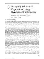
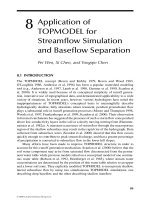
The results indicate that Huron and Sanilac counties produced the greatest ani-
mal waste loading potential per acre of land (over 30 tons per acre); Tuscola and
Lapeer counties had the second highest loading potential (20–30 tons per acre) in
the Cass River watershed (Figure 10.3). Portions of Sanilac and Tuscola counties had
animal manure loading potential of over 40 tons per acre of land annually. Distri-
bution of nitrogen and phosphate from animal manure by zip code shows a similar
pattern. Huron, Sanilac, and Lapeer counties had the highest nitrogen and phosphate
TABLE 10.2
Distribution of wind erosion potential
in the Cass River watershed.
Wind erosion potential Acres Percent
No wind erosion 257,756 44.3
Subtle wind erosion 57,069 9.8
Little wind erosion 120,131 20.7

Medium wind erosion 143,951 24.8
Severe wind erosion 2,155 0.4
Total 581,063 100.0
© 2008 by Taylor & Francis Group, LLC
122 Wetland and Water Resource Modeling and Assessment
loading potential, Tuscola County had the second highest amount, and Saginaw and
Genesee counties had the lowest loading potential in the Cass River watershed. At
the zip code level, four zip code areas (48465, 48426, 48729, and 48464) had animal
manure N production rates of greater than 150 lb/acre. Consequently, these loca-
tions can be targeted for implementation of manure management programs. This
also indicates that agricultural statistics data at the ner scale (below county level)
would reveal more useful information than would the county-level data in animal
manure management. Large livestock operations difcult to identify at county level,
could be easily identied using the 5-digit zip code level for manure management
(He and Shi 1998).
The total loading potential for the animal manure, nitrogen, and phosphate was
10 million tons, 26 tons, and 21 tons, respectively, in the Cass River watershed, aver-
aging 30 tons of animal waste, 160 lbs of nitrogen, and 130 lbs of phosphate per acre
of agricultural land (Table 10.3). The high loading potential per acre of agricultural
land makes optimal management of animal manure in the Cass River watershed nec-
essary for minimizing the pollution potential to the surface and subsurface waters.
These estimates, of course, do not include manure produced by other animals such
as sheep and poultry. Thus, it is inevitable that discrepancies exist between the actual
animal manure amount and these estimates. Users should realize the limitation of
these estimates when using them for water resources planning.
48735
48726
48475
48470
48456

48465
48427
48472
4842648729
48723
48733
48768
48744
48435
48464
48746
48483
48420
48415
48734
48722
48601
Legend
(kg/ha/year)
0–289
290–1981
1982–4019
4020–5170
5171–8838
8839–12283
12284–23821
23822–38757
48760
48741
48453

48416
48471
48727
0
Data source :
1987 U.S. Census of Agriculture
SAGINAW
TUSCOLA
HURON
SA
GINAW BAY
SANILAC
LAPEERGENESEE
FIGURE 10.3 Distribution of animal manure (in kg/ha) by zip code in the Cass River water-
shed. Data from U. S. Department of Agriculture, 1987 Census of Agriculture, Washington,
DC: U.S. Department of Agriculture, National Agricultural Statistics Service.
© 2008 by Taylor & Francis Group, LLC
Estimating Nonpoint Source Pollution Loadings 123
10.5 AGRICULTURAL CHEMICAL LOADING POTENTIAL
Agricultural chemical data from the Michigan Department of Agriculture (MDA)
were used to estimate the loading potential of agricultural chemicals (including both
fertilizers and pesticides) in the Cass River watershed. The MDA Pesticide and Plant
Pest Management Division (PPMD) maintains two databases for tracking pesticide
use: (1) restricted-use pesticide (RUP) (pesticides that could cause environmental
damage, even when used as directed), and sales-based estimates, which record all
RUP sales in the state of Michigan; and (2) survey-based estimates, which provide
estimates of pesticide use associated with each production type in a county by multi-
plying crop acreage by percentage of area treated and average application rates based
on the 1990 and 1991 agricultural chemical usage survey data. Nitrogen fertilizer
usage data were also estimated from the agricultural chemical usage survey data

at the county level (USDA National Agricultural Statistics Services 1990, 1991).
The uncertainty associated with the RUP sales-based estimates is that the loca-
tions of sales and applications of pesticides may not be the same. The problem with
the survey-based estimates is that crop production estimates and pesticide applica-
tion estimates are not available for all crops (Michigan Department of Agriculture,
1993). We used the survey-based estimates for pesticides and nitrogen fertilizer for
estimating agricultural chemical loading potential in the Cass River watershed. The
estimates were further adjusted by consulting the Michigan State University (MSU)
Cooperative Extension Service pesticide expert (Renner, personal communication
1994). These estimates were lumped together to derive the average usage of pesti-
cides per acre of cropland at the county level. They were not differentiated by their
toxic level as this project focused on estimating the loading potential of total agricul-
tural chemicals. Similarly, the usage of nitrogen fertilizers were divided by the total
acreage of application cropland to derive the average usage of nitrogen fertilizer per
acre of cropland. Average phosphate application data for all the cropland were based
on the USDA National Agricultural Statistical Service’s 1990 and 1991 eld crops
survey results at the state level (Table 10.4).
As shown in Table 10.4, approximately 15 million pounds of nitrogen and 13.5
million pounds of phosphate fertilizers, and 206,000 pounds of pesticides were
applied to cropland in the Cass River watershed annually. Although these numbers
represent the amounts applied to the crops and a major portion of these may be used
by plants, some portions of these could be transported either through surface runoff
TABLE 10.3
Estimated total amounts of animal waste, nitrogen,
and phosphate from animal waste in the Cass River
watershed based on the 1987 Census of Agriculture data.
Animal
waste
(tons)
Nitrogen

(N)
(tons)
Phosphate
(P
2
O
5
)
(tons)
9,632,000 25,700 21,180
© 2008 by Taylor & Francis Group, LLC
124 Wetland and Water Resource Modeling and Assessment
or drainage tiles to the surface waters or leached to groundwater in the watershed.
Thus, implementing best management practices in applying agricultural chemicals is
crucial for reducing the pollution potential in the Cass River watershed.
10.6 CRITICAL NONPOINT SOURCE POLLUTION AREAS
Taking into account the loading potential of soil erosion, animal manure, and agri-
cultural chemicals, it seems that the overall nonpoint source pollution potential is
highest in the Huron, Sanilac, and eastern Tuscola portions of the Cass River water-
shed. These areas, located in the upper stream of the Cass River watershed, are
mainly cropland with relatively high slope and close proximity to drains and tribu-
taries. The high fertilizer and pesticide application rate, and the large amount of
animal manure from concentrated livestock industry, and intensive cropping activi-
ties make these areas a major source of potential contamination to the surface and
subsurface waters in the Cass River watershed. In addition, as these areas are located
in the upper stream, activities in these areas will have a greater impact on the water
quality downstream.
The simulated sediment yield from AGNPS appears to be greatest in the mouth
of the Cass River near Saginaw due to the atness of the area. The larger amount
of sedimentation in the area is likely to have a negative impact on aquatic habitat. It

could also lead to elevated streambed and increased ooding frequency and damage
in the surrounding areas. These areas could be targeted for future water quality man-
agement programs for minimizing nonpoint source contamination potential.
10.7 SUMMARY
The National Oceanic and Atmospheric Administration (NOAA) Great Lakes Envi-
ronmental Research Laboratory (GLERL) and Western Michigan University are
developing a spatially distributed, physically based watershed-scale water quality
model to estimate movement of materials through point and nonpoint sources in both
surface and subsurface waters to the Great Lakes watersheds. This paper, through
TABLE 10.4
Estimated agricultural chemical loading potential
in the Cass River watershed.
County
Cropland
(acres)
Nitrogen
amount
(lbs)
Phosphate
amount
(lbs)
Pesticides
amount
(lbs)
Huron 10,164 579,348 426,888 8,284
Genesee 4,932 247,093 207,144 3,290
Lapeer 11,713 585,650 491,946 7,567
Saginaw 21,729 956,076 912,618 15,428
Sanilac 136,114 6,669,586 5,716,788 83,030
Tuscola 137,389 6,182,505 5,770,338 88,341

Total 322,041 15,220,000 13,526,000 206,000
© 2008 by Taylor & Francis Group, LLC
Estimating Nonpoint Source Pollution Loadings 125
a case study of the Cass River watershed, estimates loading potential of soil ero-
sion and sediment by water and wind, animal manure and nutrients, and agricul-
tural chemicals. The results suggest that the Cass River watershed introduces large
amounts of nutrients and sediment into the Saginaw River and Bay. Soil erosion was
up to 5 tons per acre in some agricultural land areas after a single 24-hour storm
of 3.7 inches with frequency of one in 25 years. The sediment yield was up to 145
tons per acre at the outlet of the watershed. Total nitrogen and phosphorus runoff
was higher in agricultural land. About 25% of the total land area in the Cass River
watershed was subject to medium wind erosion. The concentrated animal industry
produces approximately 10 million tons of manure, 26 tons of nitrogen, and 21 tons
of phosphate in the Cass River watershed, averaging 30 tons of manure, 160 lbs of
nitrogen, and 130 lbs of phosphate per acre of agricultural land annually. About 15
million lbs of nitrogen fertilizer, 13 million lbs of phosphate, and 206,000 lbs of pes-
ticides were used annually in the agricultural land of the Cass River watershed. Por-
tions of these fertilizers and pesticides could be transported, either through surface
runoff or drainage tiles, to the streams and groundwater in the watershed.
Agricultural statistics data at the ner scale (below county level) would reveal
more useful information than would the county-level data in estimating multiple
sources of pollutant loading potential. Governmental agencies should consider col-
lecting and tabulating relevant information at the township or zip code level to aid
environmental planning and management.
This paper estimates the loading potential of multiple sources of pollutants
but does not consider the pollutant transport through runoff processes in the entire
watershed. Work is underway to provide these estimates to the distributed large
basin runoff water quality model for simulating pollutant transport in both surface
and subsurface water in the Saginaw Bay watersheds. Such information, once veri-
ed with the Saginaw Bay water quality data, will help management agencies and

ecosystem researchers in prioritizing water quality control programs and protecting
critical sheries and wildlife habitat.
ACKNOWLEDGMENTS
This is GLERL Contribution No. 1376. Partial support from the Western Michi-
gan University Department of Geography Lucia Harrison Endowment Fund and the
Michigan State University Institute of Water Research is also appreciated.
REFERENCES
Arnold, G., R. Srinavasan, R. S. Muttiah, and J. R. Williams. 1998. Large area hydrologic
modeling and assessment. Part I. Model development. Journal of the American Water
Resources Association 34: 73–89.
Beasley, D. B., and L. F. Huggins. 1980. ANSWERS (Areal nonpoint source watershed envi-
ronment simulation)—user’s manual. West Lafayette, IN: Department of Agricultural
Engineering, Purdue University,
Beasley, R. P., J. M. Gregory, and T. R. McCarty. 1984. Erosion and sediment pollution con-
trol. 2nd ed. Ames: Iowa State University Press.
Croley, T. E., II, and C. He. 2005. Distributed-parameter large basin runoff model I: Model
development. Journal of Hydrologic Engineering (ASCE) 10:173–181.
© 2008 by Taylor & Francis Group, LLC
126 Wetland and Water Resource Modeling and Assessment
Croley, T. E., II, C. He, and D. H. Lee. 2005. Distributed-parameter large basin runoff model
II: Application. Journal of Hydrologic Engineering (ASCE) 10:182–191.
Croley, T. E., II, and C. He. 2006. Watershed surface and subsurface spatial intraows. Jour-
nal of Hydrologic Engineering (ASCE) 11:12–20.
Foster, G. R., D. C. Yoder, D. K. McCool, G. A. Weesies, T. J. Toy, and L. E. Wagner. 2000.
Improvements in science in RUSLE2. Paper No. 00-2147. ASAE, St. Joseph, MI.
Gregory, J. M 1984. Prediction of soil erosion by water and wind for various frac-
tions of cover. Transactions of the American Society of Agricultural Engineers
27:1345–1350.
He, C. 2003. Integration of GIS and simulation model for watershed management. Environ-
mental Modeling and Software 18:809–813.

He, C., and T. E. Croley II. 2005. Development of a distributed large basin operational hydro-
logic model. Control Engineering Practice (in review).
He, C., and T. E. Croley II. 2007 Application of a distributed large basin runoff model in the
Great Lakes Basin. Control Engineering Practice 15:1001–1011.
He, C., J. F. Riggs, and Y. T. Kang. 1993. Integration of geographic information systems and
a computer model to evaluate impacts of agricultural runoff on water quality. Water
Resources Bulletin 29:891–900.
He, C., and C. Shi. 1998. A preliminary analysis of animal manure distribution in Mich-
igan for nutrient utilization. Journal of the American Water Resources Association
34:1341–1354.
He, C., C. Shi, and Y. T. Kang. 1994. Modeling agricultural nonpoint source pollution poten-
tial in support of environmental decision making. East Lansing: Institute of Water
Research, Michigan State University.
He, C., C. Shi, C. Yang, and B. P. Agosti. 2001. A Windows-based GIS-AGNPS interface.
Journal of the American Water Resources Association 37:395–406.
Knisel, W. G., ed. 1980. CREAMS: A eldscale model for chemical, runoff, and erosion from
agricultural management systems, Conservation Report No. 26. Washington, DC: U.S.
Department of Agriculture, Science and Education Administration.
Leonard, R. A., W. G. Knisel, and D. A. Still. 1987. GLEAMS: Groundwater loading effects
of agricultural management systems. Transactions of the American Society of Agricul-
tural Engineers 30:1403–1418.
Lillesand, T. M., and R. W. Kiefer. 1987. Remote sensing and image interpretation. New
York: John Wiley & Sons.
Merva, G. E. 1986. Bay County wind erosion research (nal report). East Lansing: Michigan
State University, Department of Agricultural Engineering.
Michigan Department of Agriculture. 1991. Michigan Agricultural Statistics 1990, 1991.
Lansing: Michigan Department of Agriculture.
Michigan Department of Agriculture. 1993. Differential mapping of pesticide use for Michi-
gan’s state management plan. Lansing: Michigan Department of Agriculture.
Michigan Department of Natural Resources. 1988. Remedial action plan for Saginaw River

and Saginaw Bay. East Lansing: Michigan Department of Natural Resources, Surface
Water Quality Division, Great Lakes and Environmental Assessment Section.
Midwest Plan Service. 1993. Livestock Waste Facilities Handbook. 3rd ed. MWPS-18,
Midwest Plan Service, Ames: Iowa State University.
Presson, W. A. 1986. A wind erosion model to predict average soil loss for single events.
MS thesis, Department of Agricultural Engineering, Michigan State University, East
Lansing, Michigan.
Sharpley, A. N., and J. R. Williams, eds. 1990. EPIC—Erosion/productivity impact calcula-
tor, Technical Bulletin No. 1768. Washington, DC: U.S. Department of Agriculture,
Agricultural Research Service.
© 2008 by Taylor & Francis Group, LLC
Estimating Nonpoint Source Pollution Loadings 127
U.S. Department of Agriculture, National Agricultural Statistical Service. 1990. Agricul-
tural chemical usage: 1990 eld crops summary. Washington, DC: U.S. Department
of Agriculture.
U.S. Department of Agriculture, National Agricultural Statistical Service. 1991. Agricul-
tural chemical usage: 1991 eld crops summary. Washington, DC: U.S. Department
of Agriculture.
U.S. Department of Agriculture, Soil Conservation Service. 1994. State soil geographic data
base (STATSGO) data users guide. Miscellaneous Publication Number 1492, Washing-
ton, DC: U.S. Department of Agriculture.
U.S. Environmental Protection Agency. 2002. National water quality inventory 2000 report.
EPA-841-R-02-001, Washington, DC: U.S. Environmental Protection Agency.
Wischmeier, W. H., and D. D. Smith. 1978. Predicting rainfall erosion losses. Agricultural
Handbook No. 537, Washington, DC: U.S. Department of Agriculture.
Woodruff, N. P., and F. H. Siddoway. 1965. A wind erosion equation. Soil Science Society of
America Proc. 29:602–608.
Young, R. A., C. A. Onstad, D. D. Bosch, and W. P. Anderson. 1989. AGNPS: A non-point-
source pollution model for evaluating agricultural watersheds. Journal of Soil and
Water Conservation 44:168–173.

© 2008 by Taylor & Francis Group, LLC