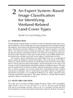
WETLAND AND WATER RESOURCE MODELING AND ASSESSMENT: A Watershed Perspective - Chapter 17 pdf

201
17
Soundscape
Characteristics
of an Environment
A New Ecological Indicator
of Ecosystem Health
Jiaguo Qi, Stuart H. Gage, Wooyeong Joo,
Brian Napoletano, and S. Biswas
17.1 INTRODUCTION
Landscape characteristics are important measures of an ecosystem’s environmental
health, as they depict spatial patterns of physical attributes of the landscape that
many organisms rely on. The visual features of a landscape, such as forest type,
density, patch size and shape, affect habitat properties that are specic to differ-
ent organisms. Change or disruption of the spatial patterns of a landscape has been
shown to impact biodiversity (Crist et al., 2004, Jeanneret et al., 2003, Sala et al.,
2000, Foley et al., 2005), ecological function (Allan, 2004, Alberti, 2005, Grigulis
et al., 2005, Battin, 2004), and ecosystem services (Tscharntke et al., 2005, Fischer
and Lindenmayer, 2007).
A suite of landscape matrices has been developed based on land use and land
cover maps derived from satellite images as a measure of landscape fragmentation.
They include, for example, patch density, Shannon diversity index, as proxies of
landscape characteristics. These matrices have been found to be important indica-
tors of an ecosystem’s biodiversity and integrity (Sala et al., 2000, Foley et al., 2005,
Fischer and Lindenmayer, 2007).
Although these landscape characteristics, often derived from analysis of remotely
sensed imagery, are important indicators of ecosystem health, they are temporally
static and do not provide a sufcient spatial resolution to observe the responses of
individual organisms to anthropogenic disturbances. The audio characteristics emit-
ted from an ecosystem, such as sounds from birds, mechanical movements, or wind
(Truax, 1999, Schafer, 1977), provide unique insight into spatial and temporal pat-

terns of ecosystem responses to human disturbances. While soundscape characteris-
tics provide complementary information to landscape characteristics, little research
has been done to fully explore the usefulness of coupling these two complementary
indicators of ecological dynamics.
© 2008 by Taylor & Francis Group, LLC
202 Wetland and Water Resource Modeling and Assessment
We dene an ecosystem’s soundscape as the physical extent of acoustic signals
and the spectral range of signal frequencies associated with an ecosystem’s biophysi-
cal processes. Truax (1999) and Schafer (1977) introduced the idea of a soundscape
in their early studies of acoustic ecology. Environmental soundscape analysis as a
complementary measure of ecosystem dynamics uniquely addresses some of the key
criteria for the establishment of ecological indices as articulated by Dale and Beyler
(2001). Soundscape analysis is a predictable measure of ecosystem stress, is antici-
patory, is integrative, and can measure disturbance. Because an ecosystem’s sound-
scape is a function of a variety of ecological variables, assessment of the soundscape
serves to integrate several variables in the measure of integrity and biocomplexity
(Thompson 2001, Holling 2001, Mueller and Kuc 2000, Porter et al., 2005). This
chapter demonstrates the capability of acoustic sensing techniques to characterize
an ecosystem’s soundscape.
17.2 ACOUSTIC SIGNAL CLASSIFICATION
Viewed in terms of information theory, the acoustic frequency spectrum is primar-
ily an information-carrying medium. An organism or force generating the acous-
tic signal acts as the encoder and transmitter, and the acoustic spectrum acts as
the medium through which the encoded signal travels. The receiver then registers
and decodes the signal (as in human conversation, for instance). The various signals
within the acoustic spectrum are commonly classied as either natural or human-
induced sounds (Schafer 1977).
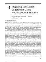
Krause (1998), in his studies of natural soundscapes, devised the term biophony
to describe the complex chorus of ambient biological sounds (biophony = biologic
and symphony), and geophony for a region’s ambient geological sounds (Figure 17.1).

Similarly, the term anthrophony refers to the human-imposed sounds (0.2–2.0 kHz).
The two primary categories, biophony and anthrophony, can be further subdivided
conceptually. Early observations led to the conclusion that signals within the bio-
phony range (2.0–11.0 kHz) can be characterized as intentional, meaning the trans-
mitter of the signal wishes to communicate information, such as mating or distress
calls, through the acoustic spectrum, or incidental, in which signals transmitted
may contain relevant information but are not dispatched for the explicit purpose of
communication.
Anthropogenic sounds can be further divided into mechanistic and oral classes.
Oral sounds are those produced by human beings themselves (i.e., talking, shout-
ing, or singing). Conversely, mechanistic signals involve sounds produced by vari-
ous forms of human-made machinery and technology. Within this class, two further
subcategories exist: stationary and temporal. Stationary refers to those signals that
impose themselves on the ambient soundscape permanently (i.e., turbulence from
air-conditioner fans), and temporal signals include the noises that move through
the soundscape over a given temporal scale (i.e., automobile or train trafc). While
this schema does not provide an absolute standard of acoustic classication, it
does provide the framework to begin characterization of acoustic signaling (see
Figure 17.1).
© 2008 by Taylor & Francis Group, LLC
Soundscape Characteristics of an Environment 203
17.3 SOUNDSCAPE ANALYSIS
17.3.1 E
COLOGICAL SOUNDSCAPES
Acoustic diversity refers to the patterns of frequency and temporal use of the acous-
tic spectrum. Biophonic complexity thereby indicates the degree to which different
vocalizing organisms utilize different niches to relay information within the spec-
trum. Specically, ecosystems with lesser degrees of human interference tend to
exhibit greater biophonic complexity in terms of frequency and periodicity utiliza-
tion. Moreover, anthropogenic interference, and more particularly temporal interfer-

ence, within a soundscape will tend to hinder organism populations by lowering
reproduction rates and increasing predation rates. Organisms make careful use of
the acoustic frequency when attempting to communicate information such as mating
potential, territory size, and potential predation. When anthropogenic interference
disrupts this communication, critical information is not relayed and the organism’s
population experiences a decline (Krause 1998). Therefore, acoustic characteristics
may serve as an ecological indicator of ecosystems.
17.3.2 DEVELOPMENT OF SOUNDSCAPE INDICATORS
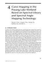
An acoustic signal is characterized by multiple physical attributes including timing,
frequency, and intensity. The data set produced by acoustic recordings and quanti-
cation is an array of acoustic intensity of contiguous, nonoverlapping frequency
bands (Figure 17.2). These data form a data matrix where the rows represent record-
ing intervals and the columns are frequency bands. A wide frequency band summa-
rizes the intensity of sound waves across a relatively wide set of frequencies, while
a narrow band restricts the range of frequency summarized. The analytical role is to
summarize patterns in covariation among the different frequency bands across the
temporal period during which the acoustic data were recorded. The most convincing
and feasible statistical method for describing such patterns of covariation in each
acoustic signature is to calculate the dominance in each frequency band and compute
their statistical distributions.
Intentional
Signaling
Incidental
Signaling
Biophony Geophony
Oral
Communications
Stationary Temporary
Mechanistic
Sounds

Anthrophony
Sound Spectrum
FIGURE 17.1 View diagram of acoustic taxonomy.
© 2008 by Taylor & Francis Group, LLC
204 Wetland and Water Resource Modeling and Assessment
In impacted ecosystems the spectral properties of acoustic signals in the environ-
ment sometimes aggregate within two primary regions of a spectrogram. The rst
region occurs at the lower frequencies of the sound spectrum. This band typically
extends from 0.2 to 1.5 kHz and consists primarily of mechanical signals (e.g., trains,
cars, air conditioners, etc.), and is therefore referred to as the anthrophonic region.
The second band of concentration begins in the range of 2 kHz and is prevalent up to
8 kHz, but may reach a higher spectral range especially when organisms communi-
cate using wider signal bandwidths (e.g., Molothrus ater) or ultrasound (e.g., bats). We
currently restrict our range to human detection to match with human auditory survey
techniques. This realm of acoustic activity consists primarily of signals generated by
biological organisms, and is therefore referred to as the biophonic region. We have
delineated this frequency band as the biological band based on our observations and
the frequency ranges referred to in the literature. These two bands correspond to two
of the three taxonomic categories of the soundscape described above, but do not cover
acoustics emanating from the physical (i.e., wind, rain, etc.) or geophonic component.
This is because the geophony, when present, occurs as a signal that is diffuse through-
out the entire spectrum. The geophony is a diffuse signal that is strongest at the lowest
frequencies, but continues with a relatively high intensity into the higher frequencies,
and its individual components are difcult to isolate and identify.
Using this structure we compute the acoustic intensity for anthrophony (F), bio-
phony (G), and geophony (L). These three acoustic ranges are then compared to the
Divided into 11
frequency bands,
each 1 kHz wide
Relative mean

intensity of sound
in each 1 kHz band
Frequency Band
Frequency Class
11 Classes, Each Class~ = 1kHz
Paris Park; July 7, 2002, 0530
Mean RSA
Acoustic Signature Map (Spectrogram)
Time (30 sec)
60
40
20
0
1234567891011
FIGURE 17.2 The acoustic frequency slicing procedure. Each sound wave le is divided
into 11 frequency bands and the relative mean intensity is calculated for each band. (See color
insert after p. 162.) Note that the 5-kHz band has the highest mean intensity across the 11
frequency bands.
© 2008 by Taylor & Francis Group, LLC
Soundscape Characteristics of an Environment 205
17.4 ASAMPLEAPPLICATION
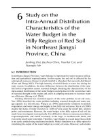
To demonstrate the usefulness of the acoustic signals as an environmental indica-
tor, sounds were recorded in Nanchang city, China (Figure 17.3) and another one
in Michigan. Nanchang Park was once a plant nursery but was transformed into a
FIGURE 17.3 A photograph of the China study site where acoustic data were collected and
analyzed in this paper.
© 2008 by Taylor & Francis Group, LLC
value of the entire signal (s). A value > 1 indicates that the concentration of acous-
tic activity in the analyzed region was greater than the value for the entire signal.
Therefore, the region with the highest value was the predominant source of acoustic

activity in the signal. For example, if the b
r
had the highest value, then biological
activity was predominant, while a larger a
r
value indicated dominant anthropogenic
activity. To emphasize the comparison of biological and anthropogenic activity, we
divided the b value by the a value to calculate r (=b/a), the ratio of biological to
anthropogenic activity.
In addition to computing the ratios of activity from our spectrumgram, we also
determined the percentage of total activity a single band contributes to the total sig-
nal. A g
p
value near 100% coincident with a b
p
value of approximately the same value
indicated that the primary signal source in the sound sample was biophony (geophysi-
cal) activity. When the a
p
value was greater than 50%, it indicated that the primary
signal source was anthrophony (anthropogenic) activity, whereas a value of b
p
greater
than 50% indicated that biophony (biological) activity was the dominant source.
206 Wetland and Water Resource Modeling and Assessment
natural reserve after it changed owners in 1996. Soon after that, the park became
one of the primary nesting and mating areas for summer migratory birds. Sound
recording ecosystems were developed and calibrated, and the sounds were recorded
between July 7 and 15, 2005 at 30-minute time intervals. The Michigan site was
located in a backyard of a private house in a rural residential area in Okemos, Michi-

gan, surrounded by forests woodlots. Acoustic recorders were placed about 40 yards
away from the house for a multiple year data collection. However, in this study, we
only used a short period of time data in July 7, 2005 that are coincident with the data
from China.
As a demonstration of the soundscape characteristics, Figure 17.4, depicts the
sound spectra of selected acoustic signals from data collected on July 5, 2005 at
7:30 p.m. local time in Nanchang (top) and on July 9, 2005 at 5:30 a.m. in Michigan
(bottom). The horizontal axis is the time (30 seconds in this case) while the y-axis is
the frequency. The brightness of the image represents the vocal strength or intensity.
The brighter the image, the intense or loud the sound is. The two spectra from Michi-
gan and Nanchang showed different acoustic patterns suggesting different biological
activities at the two sites.
The two sites also showed different proportions of biological and anthropogenic
activities. Analysis of the acoustic signals in the frequency domain (Figure 17.5)
suggest that Michigan site had more biological signals than anthropogenic activities
while the Nanchang site has almost equal biological and anthropogenic activities, as
indicated in the histograms of the frequency. Although qualitative, the Nanchang site
indeed had more human related acoustic signals as it is in the Center of the big city,
Nanchang, China, while the site in Michigan is a residential area at the outskirts of
a small city, Okemos, Michigan. The ratios of biological to anthropogenic signals
( W = G/F) of
t
he two sites are compared in Figure 17.6 and they suggest the same
results as in Figure 17.5 that the biological activities are dominant at the Michigan
site while the anthropogenic activities were dominant at the Nanchang site.
Another type of application of the acoustic sensing technology is monitoring
of bird species through pattern recognition. Once an acoustic image is generated, a
signature of a specic bird, for example, can be identied (Figure 17.7). This identi-
ed acoustic signature (training signature) can then be used in image processing to
search for similar patterns in other acoustic data, thus detecting the presence of such

bird. Once expanded in time series, one can detect and monitor bird species and
possibly population.
17.5 DISCUSSION AND CONCLUSIONS
The research results presented in this paper represent a frontier work in expanding
traditional remote sensing to acoustic sensing. The fundamental difference between
traditional remote sensing and acoustic remote sensing is that the former utilizes
electromagnetic elds while the latter relies on air for signal transmission. There-
fore, a series of questions arises that needs to be addressed. The rst one is related
to the transmission of acoustic signals—how far does the acoustic signal travel, that
is, what is the distance between the recording device and the sound of origin? This
may well depend on the location of the sensor (in forested lands, grasslands, open
© 2008 by Taylor & Francis Group, LLC
Soundscape Characteristics of an Environment 207
urban lands) and its surrounding physical environment. One may record the acoustic
signal of a bird, for example, but may also realize that the bird was just ying over
rather than inhabiting the landscape where the sensor is placed. Unlike traditional
remote sensing where each pixel is associated with a xed physical dimension of
a landscape (e.g., pixel size), acoustic signals do not have a xed range of physical
dimension, as the recorded signals will vary depending on the sensor’s sensitivity,
distance of sound of origin, and physical characteristics of the environment (windy
days, or densely forested environment, for example). Therefore, interpretation of
10000
8000
6000
4000
2000
10000
8000
6000
4000

2000
5 sec 10 Sec 15 Sec 20 Sec 25 Sec
5 sec 10 Sec 15 Sec 20 Sec 25 Sec 30 Sec
FIGURE 17.4 Sound spectra of selected acoustic signals from data collected on July 5,
2005 at 7:30 p.m. local time in Nanchang (top) and on July 9, 2005 at 5:30 a.m. in Michigan
(bottom). (See color insert after p. 162.)
© 2008 by Taylor & Francis Group, LLC
208 Wetland and Water Resource Modeling and Assessment
acoustic signals is best achieved when considering the physical environment or land-
scape properties.
The use of acoustic signals as an ecological indicator is only feasible for infer-
ring ecological information of those species that generate vocal signals. Amphib-
ians and mammals, for example, do not generate sounds that can be recorded with
traditional recording devices. Thus, at this time, we can only infer information about
vocal species.
The temporal characteristics of acoustic signals are critical components of any
interpretation. Unlike the physical environment of a landscape, the soundscape is a
very dynamic eld that varies considerably within a short period of time. Diurnal
behavior of many bird species would result in a strong biological frequency in a
soundscape in the early morning, while crickets are active in the evening. These
0
5
10
15
20
L2 L3 L4 L5 L6 L7 L8 L9 L10 L11
Acoustic Frequency Bands (kHz)
L2 L3 L4 L5 L6 L7 L8 L9 L10 L11
Acoustic Frequency Bands (kHz)
Acoustic Intensity

0
5
10
15
20
25
Acoustic Intensity
FIGURE 17.5 Frequency distributions of the acoustic spectra from Figure 17.4.
© 2008 by Taylor & Francis Group, LLC
Soundscape Characteristics of an Environment 209
temporal characteristics need to be considered when attempting to capture the bio-
logical soundscape of these species.
The analytical methods used in this paper are only examples in analyzing acous-
tic signals and there are other ecological indicators that can be derived from acous-
tic signals. However, this paper represents the rst involving remote sensing that
utilizes frequencies or wavelengths that can only be transmitted through a physical
medium such as air. Nevertheless, the expansion of the remote sensing concept to
acoustic signal analysis has provides complementary and useful information about
the ecological characteristics of an environment. When applied spatially and tempo-
rally across a landscape, much more comprehensive information can be inferred. For
example, a network of sensors in a city with simultaneous measurements of acoustic
signals may provide not only information on ecological characteristics, but also a
0
5
10
15
20
25

αβγ

China
U.S.
FIGURE 17.6 Calculated alpha ( ), beta ( ), and their ratios using the data from
Figure 17.5.
Sonogram
Chipping Sparrow
Frequency
Time
0
11
0
30
FIGURE 17.7 Demonstration using acoustic signals in time series analysis to identify bird
species and population. (See color insert after p. 162.)
© 2008 by Taylor & Francis Group, LLC
a
b
210 Wetland and Water Resource Modeling and Assessment
quantitative measure of human-induced noise levels across the entire city, which is
a very valuable indicator of the environmental quality of the city. With long-term
measurements of such acoustic signals, one may further understand environmental
degradation processes.
Finally, this technology is relatively inexpensive compared with traditional
remote sensing devices, and therefore can be deployed to obtain long-term and spa-
tially distributed data. Furthermore, the operation of recording devices is relatively
simple and inexpensive in comparison with optical remote sensing devices, thus pro-
viding a convenient technology for broader applications.
ACKNOWLEDGMENTS
The Great Lakes Fisheries Trust provided support for investigating acoustic signals
as part of a grant entitled Ecological Assessment of the Muskegon River Water-

shed awarded to a consortium of investigators. This work was also supported by the
NASA grant (NNG05GD49G) and by a grant at IGSNRR of Chinese Academy of
Sciences (Human Activities and Ecosystem Changes). We want to thank Nathan Tor-
bick for installation of the recording devices and data recording, Liu Ying at Jiangxi
Normal University for his assistance in data acquisition, and Weitao Ji at the Poyang
Lake Station for allowing the authors to use their facilities at Tiangxing Yuan Park
and Poyang Lake.
REFERENCES
Alberti, M., 2005, The effects of urban patterns on ecosystem function. International
Regional Science Review Vol. 28, No. 2, 168–192
Allan, J. David, 2004, Landscapes and riverscapes: the inuence of land use on stream eco-
systems. Annual Review of Ecology, Evolution, and Systematics Vol. 35:257–284
Battin, J., 2004, When good animals love bad habitats: Ecological traps and the conservation
of animal populations. Conservation Biology 18, 1482–1491.
Crist, P. J. , T. W. Kohley and J. Oakleaf, 2004. Assessing land-use impacts on biodiversity
using an expert systems tool. Landscape Ecology Vol. 15, no. 1, pp. 1–84.
Dale, V. H., and S. C. Beyler. 2001. Challenges in the development and use of ecological
indicators. Ecological Indicators 1:3–10.
Fischer, Joern and David B. Lindenmayer, 2007. Landscape modication and habitat frag-
mentation: A synthesis. Global Ecology and Biogeography 16 (3), 265–280.
Foley, J.A., R. DeFries, G.P. Asner, C. Barford, G. Bonan, S.R. Carpenter, F.S. Chapin,
M.T.Coe, G.C. Daily, H.K. Gibbs, J.H. Helkowski, T. Holloway, E.A. Howard,
C.J. Kucharik, C. Monfreda, J.A. Patz, I.C. Prentice, N. Ramankutty, and P.K. Snyder,
2005. Global consequences of land use. Science 309, 570–574.
Grigulis, Karl, Sandra Lavorel, Ian D. Davies, Anabelle Dossantos, Francisco Lloret, Mont-
serrat Vilà, 2005. Landscape-scale positive feedbacks between re and expansion of
the large tussock grass, Ampelodesmos mauritanica in Catalan shrublands. Global
Change Biology 11(7), 1042–1053.
Holling, C. S. 2001. Understanding the complexity of economic, ecological, and social sys-
tems. Ecosystems 4:390–405.

Jeanneret P., B. Schüpbach, H. Luka, and W. Büchs 2003. Quantifying the impact of land
-
scape and habitat features on biodiversity in cultivated landscapes. Biotic indicators for
biodiversity and sustainable agriculture 2003,Vol.98,no. 1–3, pp.311–320.
© 2008 by Taylor & Francis Group, LLC
Soundscape Characteristics of an Environment 211
Kime, N. M., W. R. Turner, and M. J. Ryan. 2000. The transmission of advertisements calls
in Central American frogs. Behavioral Ecology 11:71–83.
Krause, B. 1998. Into a wild sanctuary: A life in music and natural sound. Berkeley, CA:
Heyday Books.
Mueller, R., and R. Kuc. 2000. Foliage echoes: A probe into the ecological acoustics of bat
echolocation. Journal of the Acoustical Society of America 108:836–845.
Naguib, M. 1996. Ranging by song in Carolina Wrens Thryothorus ludovicianus: Effects of
environmental acoustics and strength of song degradation. Behaviour 133:541–559.
Penna, M. a. R. S. 1998. Frog call intensities and sound propagation in the South American
temperate forest region. Behavioral Ecology and Sociobiology 42:371–381.
Porter, J., P. Arzberger, H.W. Braun, P. Bryant, S. Gage, T. Hansen, P. Hanson, C.C. Lin, F.
P. Lin, T. Kratz, W. Michener, S. Shapiro, and T. Williams, 2005. BioScience Vol. 55,
no. 7, pp. 561–572
Sala, O. E., F.S. Chapin, J.J. Armesto, E. Berlow, J. Bloomeld, R. Dirzo, E. Huber-Sanwald,
L.F. Huenneke, R.B. Jackson, A. Kinzig, R. Leemans, D.M. Lodge, H.A. Mooney,
M. Oesterheld, N.L. Poff, M.T. Sykes, B.H. Walker, M. Walker, and D.H. Wall. 2000.
Global biodiversity scenarios for the year 2100. Science 287, 1770–1774.
Schafer, R. M. 1977. The soundscape: Our sonic environment and the tuning of the world.
Rochester, VT: Destiny Books.
Skole, D., and C. Tucker. 1993. Tropical deforestation and habitat fragmentation in the Ama-
zon: Satellite data from 1978 to 1988. Science 260:1905–1910.
Snedden, W. A., M. D. Greeneld, and Y. Jang. 1998. Mechanisms of selective attention in
grasshopper choruses: Who listens to whom? Behavioral Ecology and Sociobiology
43:59–66.

Thompson, J. N. 2001. Frontiers of ecology. BioScience 51:15–24.
Truax, B. 1999. Handbook for acoustic ecology. Burnaby, BC: Cambridge Street Publishers.
Tscharntke, T., A. M. Klein, A, Kruess, I. Steffan-Dewenter, and C. Thies, 2005. Landscape
perspectives on agricultural intensication and biodiversity - ecosystem service man-
agement. Ecology Letters 8 (8), 857–874.
© 2008 by Taylor & Francis Group, LLC